# The Voronoi War: AI Beats the Prophet
[Authoritative PDF](paper.pdf) · Markdown reading copy
Sariel Har-Peled
### **Abstract**
A player observes sites, say in the unit square, arriving one at a time and must decide immediately and irrevocably whether to accept each one, keeping at most one. The payoff is the area of the chosen site’s cell in the Voronoi diagram of all the sites. The prophet sees all the input in advance and takes the largest cell. The author introduced this game recently, and gave a constant approximation for uniform random sites.
This writeup explores many variants of this game. Under a minor variation of the sampling model, we achieve a $`1+\varepsilon`$ approximation with high probability for any fixed $`\varepsilon> 0`$. In contrast, for arbitrary fixed sites arriving in random order, we present a strategy that achieves an $`O(\log n)`$ approximation with constant probability. Surprisingly, there are configurations where the expected competitive ratio is $`\Omega (\log n/\log \log n)`$, even when the player may make $`\sqrt n`$ choices.
The research and writing were done by the AI systems ChatGPT and Claude Fable. The human contribution was minimal.
## 1 Introduction
### 1.1 The Voronoi selection game
Consider the following online game \[[Har26](#X0-h-pvd-26)\]: A sequence of $`n`$ sites in the unit square is revealed one site at a time, and the player knows $`n`$ in advance. When a site appears, the player may accept it. The decision is immediate and irrevocable, and a site that is passed over is gone for good. Only one site may be accepted. The reward is determined after the whole sequence has arrived: it is the area of the cell of the accepted site in the Voronoi diagram of *all* $`n`$ sites, accepted or not. Opposite sides of the square are identified, so the domain is a flat torus and there are no boundary effects.
The adversarial analysis of the game is done against the *prophet*, who sees the whole input in advance and takes the site with the largest final cell. The question is how much of the prophet’s area an online player can secure. A strategy is an $`\alpha`$-approximation if its payoff is at least a $`1/\alpha`$ fraction of the largest final cell, and it is $`\alpha`$-competitive in expectation if the same holds for the expected values. Precise definitions are given in [Section 2](#fixedsize-selection-and-the-input-models).
What makes the game hard is that the value of a site is not known when it arrives. An arriving site has a visible cell in the diagram of the sites seen so far, but every later site can only shrink that cell. In the secretary problem, the classical model of irrevocable online choice, the quality of a candidate is fixed once it is observed, see Ferguson \[[Fer89](#X0-f-wssp-89)\] for the history of that problem. Here the quality of a choice keeps deteriorating after the choice is made. The original paper offers land speculation as a metaphor: a plot bought early may lose most of its value when the neighbors build around it \[[CD22](#X0-cd-rofl-22)\]. Waiting reveals more of the eventual competition, but a site that has been passed over cannot be recovered.
**The original result.** For $`n`$ independent uniform sites, Har-Peled \[[Har26](#X0-h-pvd-26), Section 4\] gave a strategy whose payoff is a constant fraction of the largest final cell with probability tending to one. The largest cell has area $`\Theta (\log n/n)`$. The strategy ignores all but a final suffix of about $`\sqrt n\log n`$ arrivals, and then accepts the first site in the suffix with no earlier site within distance $`\Theta (\sqrt {\log n/n})`$. The analysis shows that many sites have cells within a constant factor of the largest one, so one of them appears in the suffix, and that the few remaining arrivals are unlikely to spoil it. The constant in the approximation was not determined, and nothing was proved beyond uniform sampling with a known number of sites.
**Prophet inequalities.** A prophet inequality compares the expected payoff of a stopping rule with the expected maximum of a sequence of independent random values; the classical results of Krengel and Sucheston \[[KS78](#X0-ks-sapfv-78)\] and Samuel-Cahn \[[Sam84](#X0-s-ctsrm-84)\] show that a factor of two is achievable and tight. The subject has a large literature, surveyed by Hill and Kertz \[[HK92](#X0-hk-spiost-92)\] and, for its connections to pricing and mechanism design, by Lucier \[[Luc17](#X0-l-evpi-17)\] and Correa et al. \[[CFH+19](#X0-cfhov-rdpi-19)\]. In all those models the value of an item is fixed once it is revealed. The closest precedent for a payoff that deteriorates after the decision is the rank version of the secretary problem, where the payoff of the chosen item is its rank among all $`n`$ items, so every later arrival that beats it worsens the payoff. Chow et al. \[[CMRS64](#X0-cmrs-osbrr-64)\] solved the version where only relative ranks are observed; in the full-information version, known as *Robbins’ problem*, the items are independent uniform numbers in $`[0,1]`$, and the optimal expected rank is still unknown \[[BF93](#X0-bf-merwfi-93), [Bru05](#X0-b-wikarp-05)\]. Apart from that problem, we are not aware of prior work in which the payoff of a selected item keeps deteriorating because of items that arrive afterwards, which is the defining feature of the game studied here.
**Related games and tools.** In the Voronoi game of Ahn et al. \[[ACC+04](#X0-accgo-cflvg-04)\] and Cheong et al. \[[CSLM04](#X0-chlm-orvg-04)\], two players insert sites into a diagram and compete for total area. Boppana et al. \[[BHMM16](#X0-bhmm-vcg-16)\] study equilibria when each player chooses among a few given locations. Those games have complete information, and the difficulty is strategic rather than informational. Secretary problems on graphs and partial orders have also been studied; see Kubicki and Morayne \[[KM05](#X0-km-gtgsp-05)\]. On the geometric side, the Voronoi diagram of random sites is a classical object of stochastic geometry \[[OBSC00](#X0-obsc-stcav-00), [CSKM13](#X0-cskm-sga-13)\]. The specific results used below are (i) the theorem of Hug et al. \[[HRS04](#X0-hrs-lpvc-04)\], (ii) a large Poisson–Voronoi cell is nearly a disk, and (iii) the stopping identity for random-order arrivals of Mauras et al. \[[MMR24](#X0-mmr-osiv-24)\].
### 1.2 Our results
**Matching the prophet for Poisson input.** Our main result removes the constant from the original approximation. This requires us to change the sampling model slightly. Consider a uniform Poisson sample on the unit square with torus topology: the number of sites is $`N\sim \operatorname {Poisson}(\lambda )`$, and conditional on $`N`$ the sites are independent, uniform, and presented in random order. The player knows the intensity $`\lambda`$ and sees that a site is the $`t`$th arrival, but is told neither $`N`$ nor a clock reading, which would reveal how much of the stream remains. [Theorem 3.2](#x1-190022) gives an explicit one-choice rule whose payoff $`Y`$ satisfies
```math
{\mathbb{P}}\left[ Y\geq M/(1+\varepsilon ) \right]\to 1 \qquad \text {as }\lambda \to \infty ,
```
for every fixed $`\varepsilon >0`$, where $`M`$ is the largest final cell. Thus the prophet’s advantage vanishes in probability[1](#fn1x0) .
The rule has the same shape as the original one: reject a prefix, then accept the first site with an empty disk of a prescribed radius around it. The difference is quantitative. [Theorem 3.2](#x1-190022) also shows that the largest cell is asymptotic to $`\log \lambda /(4\lambda )`$ in probability, with the upper bound coming from [Lemma 3.4](#x1-220074). That bound rests on the exponential tail, with rate $`4`$, of the area of the cell of a site inserted at the origin of a unit-intensity planar Poisson process ([Lemma 3.3](#x1-220013)); scaling to intensity $`\lambda`$ gives the area scale $`\log \lambda /(4\lambda )`$. We deduce the tail from the roundness theorem of \[[HRS04](#X0-hrs-lpvc-04)\] and also prove it from scratch in [Appendix A](#an-elementary-proof-of-the-largecell-tail). An empty disk of radius $`R`$ around a site certifies that its final cell has area at least $`\pi R^2/4`$. The radius is chosen so that this certified area is within a factor $`1-o(1)`$ of $`\log \lambda /(4\lambda )`$, while [Lemma 3.5](#x1-230015) shows that polylogarithmically many sites still have such an empty disk. The length of the rejected prefix is set from $`\lambda`$ alone, so that with high probability a certificate appears after it and only about $`\lambda /\log ^2\lambda`$ sites arrive later.
**Known distributions in one dimension.** Beyond uniform sampling, the way the input is provided matters a great deal. For $`n`$ independent sites from any known non-atomic distribution on the circle, [Theorem 3.11](#x1-3600111) gives a one-choice strategy that is constant-competitive in expectation and achieves a constant-factor approximation with constant probability. The strategy selects only after the first half of the arrivals. Its key device is a geometric length scale, computed from the distribution and $`n`$ through a dyadic partition, that controls the prophet’s expected payoff. The strategy then monitors disjoint intervals at that scale, each activated at its own time so that the expected number of later arrivals into it is bounded. The constant is large and was not optimized.
**A factor-two barrier.** For smooth densities on the circle or in the plane, no strategy can do much better than a factor of two. [Theorem 3.6](#x1-280026) constructs, for each sample size, a known $`C^\infty`$ density with the following property: every strategy that may select polylogarithmically many sites and keep the best of them fails, with probability tending to one, to obtain any fixed fraction larger than one half of the largest final cell, and its expected payoff is at most $`(1/2+o(1))`$ times the expected optimum. The density concentrates its mass in tiny bumps around a regular grid, so that a site alone in its bump owns a full grid cell while a site sharing its bump owns at most half; the player cannot tell early which bumps will end up with a single site. A matching one-choice strategy achieves factor $`2+o(1)`$ on this family ([Proposition 3.10](#x1-3500110)): it waits until near the end, records the bumps holding exactly one site so far, and accepts the first later arrival into one of them; with high probability that bump ends with two sites, each owning about half a grid cell. Whether every known planar distribution admits a constant expected competitive ratio remains open.
**Fixed sites in random order.** Suppose now that an adversary fixes the sites and only their arrival order is random. One choice still obtains an $`O(\log n)`$ approximation with constant probability ([Theorem 4.3](#x1-430013)), and this is nearly tight: [Theorem 4.4](#x1-440014) exhibits inputs on which the expected competitive ratio is $`\Omega (\log n/\log \log n)`$, even if the player may select $`\sqrt n`$ sites and keep the best of them! The competitive bound being close to tight in this case is quite surprising.
For larger budgets, [Theorem 4.5](#x1-450015) quantifies the tradeoff between the number of selections and the achievable ratio: when $`n/b\to \infty`$, the cluster construction gives a planar input with expected payoff fraction $`O(\log \log (n/b)/\log (n/b))`$, and [Corollary 4.6](#x1-470016) concludes that constant expected competitiveness for arbitrary fixed planar sites requires, and is achieved by, $`\Theta (n)`$ selections. In the other direction, write $`M_2`$ for the second-largest final cell and $`\Gamma =M/M_2`$ for the gap of the optimum. [Theorem 4.7](#x1-480017) shows that the greedy rule, which accepts every arrival whose cell in the diagram of the sites seen so far is largest, captures a unique optimum with $`O(\log n)`$ selections and probability bounded away from zero as soon as $`\Gamma`$ is of order $`\log n`$, so the logarithmic gap in the lower-bound instances is the right scale.
The one-choice strategy behind the $`O(\log n)`$ bound waits for an arrival whose cell in the diagram of the sites seen so far, its *current cell*, is the largest. It samples a random location in a large triangle inside that cell and then, with a fair coin, either accepts the arriving site or searches the later arrivals for the location’s final owner. The key geometric fact is that only $`O(\log n)`$ final cells can meet that triangle. The lower bounds delete a few sites from a regular configuration and show that the player cannot tell, until it is too late, which sites are missing.
**The missing-vertex game.** The informational obstacle behind these lower bounds can be isolated in a purely combinatorial game. One vertex of a known graph is hidden, the others arrive in random order, and the player has a single irrevocable guess: upon an arrival, it may name one unseen neighbor of the arriving vertex as the hidden one. [Lemma 4.9](#x1-510019) shows that the optimal rule waits until no two unseen vertices are adjacent and then guesses, and [Proposition 4.12](#x1-5400112) expresses the optimal success probability through the numbers of independent sets. For the cycle on $`N`$ vertices the answer is $`(\sqrt \pi +o(1))/\sqrt N`$ ([Theorem 4.10](#x1-5200110)), and for every $`d`$-regular graph with $`1\leq d=o(N)`$ it is $`(\sqrt {\pi /2}+o(1))\sqrt {d/N}`$ ([Theorem 4.13](#x1-5400513)). The square-root scale has a simple source: with $`k`$ vertices still unseen, a $`d`$-regular graph has about $`dk^2/(2N)`$ edges among them, so the last unseen edge disappears when $`k`$ is of order $`\sqrt {N/d}`$, and a guess made then succeeds with probability about $`1/k`$. [Lemma 4.11](#x1-5300111) translates the cycle result into a bound on exact selection in the Voronoi game when one site is deleted from a regular circle grid.
[Table 1](#summary-of-the-results-y-is-the-players-payoff-m-the-largest-final-cell-m2-the-second-largest-mm2-and-n-the-number-of-sites-b-0-and-0-are-fixed-and-c-is-an-absolute-constant) collects these results.
| Input | Choices | Guarantee | Where |
|----|----|----|----|
| Uniform Poisson, known $`\lambda`$, hidden count | $`1`$ | $`Y\geq M/(1+\varepsilon )`$ with probability $`\to 1`$ | [Theorem 3.2](#x1-190022) |
| Any known non-atomic law on the circle | $`1`$ | $`{\mathbb{E}}\left[ Y \right]\geq {\mathbb{E}}\left[ M \right]/7000`$; constant factor with constant probability | [Theorem 3.11](#x1-3600111) |
| A constructed smooth-density family, circle or plane | $`(\log n)^{B}`$ | $`{\mathbb{P}}\left[ Y\geq M/\alpha \right]\to 0`$ for fixed $`\alpha <2`$; $`{\mathbb{E}}\left[ Y \right]\leq (1/2+o(1)){\mathbb{E}}\left[ M \right]`$ | [Theorem 3.6](#x1-280026) |
| That same family | $`1`$ | $`Y\geq M/(2+o(1))`$ with probability $`\to 1`$ | [Proposition 3.10](#x1-3500110) |
| Fixed planar sites, random order | $`1`$ | $`Y\geq cM/\log n`$ with constant probability | [Theorem 4.3](#x1-430013) |
| Fixed circle or planar sites, random order | $`\leq \sqrt n`$ | $`{\mathbb{E}}\left[ Y \right]/M=O(\log \log n/\log n)`$ for some input | [Theorem 4.4](#x1-440014) |
| Fixed planar sites, random order | $`b`$ | $`{\mathbb{E}}\left[ Y \right]/M=O(\log \log (n/b)/\log (n/b))`$ for some input when $`n/b\to \infty`$; $`\Theta (n)`$ choices needed | [Corollary 4.6](#x1-470016) |
| Fixed planar sites, random order, unique optimum with gap $`\Gamma`$ | $`O(\log n)`$ | optimum selected with probability $`\geq e^{-c\log n/\Gamma }-2/n`$ | [Theorem 4.7](#x1-480017) |
| Missing vertex, cycle $`C_N`$ | $`1`$ guess | success $`(\sqrt \pi +o(1))/\sqrt N`$ | [Theorem 4.10](#x1-5200110) |
| Missing vertex, $`d`$-regular graph, $`1\leq d=o(N)`$ | $`1`$ guess | success $`(\sqrt {\pi /2}+o(1))\sqrt {d/N}`$ | [Theorem 4.13](#x1-5400513) |
Table 1: Summary of the results. $`Y`$ is the player’s payoff, $`M`$ the largest final cell, $`M_2`$ the second largest, $`\Gamma =M/M_2`$, and $`n`$ the number of sites; $`B\geq 0`$ and $`\varepsilon >0`$ are fixed, and $`c`$ is an absolute constant.
**Two sources of randomness.** The results above use randomness in two different ways. In the sampling models, the final diagram itself is random and its law is known to the player. In the random-arrival model, the diagram is fixed but unknown, and only the order is random. [Section 2](#fixedsize-selection-and-the-input-models) specifies the information available to the player in each model and distinguishes expected competitiveness from approximation with high probability. The Poisson theorem concerns a hidden random count; the other sampling results concern a known fixed count.
**AI collaboration.** The new results were obtained in a collaboration between the author and two AI systems, starting from the original paper. ChatGPT generated and refined many of the proof arguments, explored variants and counterexamples, searched the literature, and drafted the manuscript. Claude Fable reviewed the manuscript for correctness and rewrote several proofs and this introduction for clarity. The human contribution was minimal—the author posed the problems and constructions, including the Poisson game with a hidden count, supplied proof ideas, found and corrected errors, and directed the work.
**Organization.** [Section 2](#fixedsize-selection-and-the-input-models) defines the models. [Section 3](#selection-under-known-sampling-distributions) treats known sampling distributions: the Poisson result, the factor-two barrier, and the one-dimensional theorem. [Section 4](#random-arrival-and-missing-vertices) treats fixed sites in random order and the missing-vertex game. [Appendix A](#an-elementary-proof-of-the-largecell-tail) contains the elementary proof of the Poisson tail estimate.
## 2 Fixed-size selection and the input models
In the models of this section the player knows the sample size in advance. The Poisson variant, defined separately in [Section 3.1](#a-poisson-sample-matching-the-prophet), replaces that size by a known intensity and an undisclosed random count. [Table 2](#the-input-models-in-every-model-the-payoff-is-the-largest-final-cell-in-area-or-length-among-the-accepted-sites-and-the-benchmark-is-the-largest-final-cell-of-the-whole-input) summarizes what is random and what the player knows in each model. In the table, $`D`$ is the circle or the unit square with torus topology, $`\mu _D`$ its length or area measure, $`n`$ the number of arrivals, $`b`$ the selection budget, and $`F`$ the sampling law; the formal definitions follow.
| Model | What is random | What the player knows |
|----|----|----|
| Random arrival | The order of $`n`$ sites fixed by an adversary. | $`D`$, $`n`$, the budget $`b`$; not the sites. |
| Random sample | $`n`$ independent sites from a non-atomic law $`F`$ on $`D`$, revealed in sampling order. | $`D`$, $`n`$, $`b`$, and $`F`$ exactly. |
| Uniform sample | As above with $`F=\mu _D`$. | $`D`$, $`n`$, $`b`$. |
| Smooth sample | As above with $`F`$ having a $`C^\infty`$ density, which may vanish and may depend on $`n`$. | $`D`$, $`n`$, $`b`$, and the density. |
| Uniform Poisson ([Section 3.1](#a-poisson-sample-matching-the-prophet)) | $`N\sim \operatorname {Poisson}(\lambda )`$ uniform sites on $`\mathbb T^2`$ in random order. | $`\lambda`$ and the arrival indices; neither $`N`$ nor arrival times. |
Table 2: The input models. In every model the payoff is the largest final cell, in area or length, among the accepted sites, and the benchmark is the largest final cell of the whole input.
Problem 2.1 (Voronoi selection). The domain $`D`$ is either the circle $`\mathbb T=[0,1)`$ of length one, with distances measured modulo $`1`$, or the unit square with torus topology, $`\mathbb T^2=[0,1)^2`$, with distances measured modulo $`1`$ in each coordinate. Write $`d_D`$ for this distance and $`\mu _D`$ for length or area, so that $`\mu _D(D)=1`$. The *circle* and *planar* versions below refer to these two domains.
The player knows $`D`$, the number $`n\geq 1`$ of sites, and a budget $`1\leq b\leq n`$. Sites $`p_1,\ldots ,p_n`$ arrive one at a time. On seeing $`p_t`$, the player must immediately and irrevocably accept or reject it, using the observed history and independent randomness. At most $`b`$ sites may be accepted, and rejected sites cannot be recalled. All $`n`$ sites remain competitors in the final diagram. The default is one choice, $`b=1`$; a $`b`$*-choice* variant allows the stated larger budget. There is no computational restriction.
For a nonempty finite set $`Q\subset D`$ and $`p\in Q`$, put
```math
V_Q(p)=\{x\in D:d_D(x,p)\leq d_D(x,q)\text { for all }q\in Q\}, \quad v_Q(p)=\mu _D(V_Q(p)).
```
Cell boundaries have measure zero and do not affect payoffs. Ties for the largest cell, and any other ties a strategy encounters, are broken by a fixed deterministic rule. Write $`P_t=\{p_1,\ldots ,p_t\}`$, $`P=P_n`$, and $`v(p)=v_P(p)`$. For the accepted set $`S`$, the payoff and benchmark are
```math
Y=\max _{p\in S}v(p),\qquad M=\max _{p\in P}v(p),
```
with $`Y=0`$ if $`S=\emptyset`$. Thus even several choices compete with the best single final cell. Payoff is geometric measure, regardless of the input distribution. The input law and the player’s prior information are specified by one of the models below: random arrival, or a random sample from a known law, with uniform and smooth laws as special cases.
On the torus we often work with the *periodic lift* $`Q+\mathbb Z^2`$ of a site set $`Q\subset \mathbb T^2`$. Torus and Euclidean distances agree for pairs of points at Euclidean distance at most $`1/2`$, hence inside any disk of radius at most $`1/4`$, and the torus cell $`V_Q(p)`$ is the projection of the Euclidean cell of a lift of $`p`$ in $`Q+\mathbb Z^2`$, a convex polygon contained in $`p+[-1/2,1/2]^2`$; the projection is one-to-one apart from boundaries and preserves area.
Definition 2.2 (Random arrival). For the [Voronoi selection problem](#x1-150021) on either domain, an adversary fixes $`n`$ distinct sites $`P\subset D`$. They are then presented in a uniformly random permutation, independent of the player’s randomness. The player knows $`D,n,b`$, but not $`P`$. In an impossibility result we may, when explicitly stated, tell the player a family of candidate inputs containing $`P`$; which member is the actual input remains unknown. The guarantee is required for every fixed $`P`$.
Definition 2.3 (Random sample). In the [Voronoi selection problem](#x1-150021), the sites $`p_1,\ldots ,p_n`$ are independent samples from a known non-atomic probability measure $`F`$ on $`D`$, revealed in their sampling order. The player knows $`D,n,b,F`$ in advance and may use exact probabilities of measurable regions. The measure $`F`$ may depend on $`n`$ and need not have a density. Non-atomicity ensures that the sites are distinct almost surely. An algorithm may depend on $`F`$; its stated universal constants do not.
Definition 2.4 (Uniform random sample). This is the special case of the [random-sample model](#x1-150063) in which $`F=\mu _D`$: sites are independent and uniform on the entire domain, the circle or the unit square. Uniform sampling from only a proper subregion belongs to the general random-sample model, since payoffs are measured on the whole domain.
**Guarantees and variants.** In all these models, a strategy is *expected* $`\alpha`$*-competitive* if $`{\mathbb{E}}\left[ Y \right]\geq {\mathbb{E}}\left[ M \right]/\alpha`$. For random arrival, $`M`$ is fixed and only the permutation and strategy are random. For either sampling model, both $`Y`$ and $`M`$ are evaluated on the same realized sample; this ratio of expectations is distinct from $`{\mathbb{E}}\left[ Y/M \right]`$. Approximation success means $`Y\geq M/\alpha`$, and exact selection success means $`Y=M`$. Since $`n`$ is known, a strategy that has not yet selected can always accept the last arrival; we use this fallback without further comment. Absolute constants are written $`c`$, or $`c_1,c_2,\ldots`$ when one argument needs several, with the numbering restarted in each result; they depend on nothing unless stated. Write $`B(x,r)`$ for the open disk of radius $`r`$ around $`x`$, in the metric of the domain or of the plane as the context says; all logarithms are natural. For a real $`u`$ and an integer $`j\geq 0`$, write $`(u)_j=u(u-1)\cdots (u-j+1)`$, with $`(u)_0=1`$.
Definition 2.5 (Smooth random sample). Here $`F`$ has a known $`C^\infty`$ density with respect to $`\mu _D`$. All other assumptions are those of the [random-sample model](#x1-150063). The density may vanish and may depend on $`n`$; no common positive lower bound or finite upper bound is imposed.
## 3 Selection under known sampling distributions
### 3.1 A Poisson sample: matching the prophet
Definition 3.1 (Uniform Poisson sampling). The domain is the unit square with torus topology, $`\mathbb T^2`$, as in [Voronoi selection](#x1-150021), with its distance $`d_D`$ and area measure $`\mu _D`$. The player knows an intensity $`\lambda >0`$. Draw $`N\sim \operatorname {Poisson}(\lambda )`$ and, conditional on $`N`$, draw $`N`$ independent uniform sites. Reveal the sites in uniformly random order. The player sees their locations and their arrival indices, but neither $`N`$ nor arrival times. Upon each arrival, the player may select that site irrevocably, using at most one selection. No selection is permitted after the stream ends.
For the complete sample $`P`$, the cells $`V_P(p)`$ and their areas $`v(p)`$ are as in [Voronoi selection](#x1-150021). The payoff $`Y`$ is $`v(p)`$ for the selected site $`p`$, or zero if no site is selected. The prophet receives $`M=\max _{p\in P}v(p)`$, with $`M=0`$ when $`N=0`$. Probabilities include both the sample and its arrival order.
The rule below uses only a count and a nearest-neighbor query.
**The rule.** For $`\lambda`$ large enough that $`\log \lambda >6\log \log \lambda`$, set
```math
L=\log \lambda ,\qquad k=\left \lfloor \lambda -\frac {\lambda }{L^2}\right \rfloor , \qquad R=\sqrt {\frac {L-6\log L}{\pi \lambda }}.
\tag {1}
```
Reject the first $`k`$ sites. Thereafter, select the first site with no earlier site at distance less than $`R`$. If there is no such arrival, select nothing. For the bounded range of intensities where these parameters are inapplicable, select the first arrival, if any.
**Theorem 3.2 (Poisson selection).** *In the* [*uniform Poisson sampling setting*](#x1-180011)*, the rule of* [Eq. (1)](#x1-19001r1) *satisfies, as* $`\lambda \to \infty`$*,*
```math
{\mathbb{P}}\left[ Y\ge \frac {\log \lambda -6\log \log \lambda }{4\lambda } \right]=1-O\!\left (\frac 1{\log \lambda }\right ).
```
*Moreover,*
```math
\frac {4\lambda M}{\log \lambda } \xrightarrow {\mathrm p}1, \qquad \frac {Y}{M}\xrightarrow {\mathrm p}1,
```
*where the second ratio is defined to be* $`1`$ *when* $`N=0`$*. In particular, the same rule gives a* $`(1+\varepsilon )`$ *approximation with probability tending to one for every fixed* $`\varepsilon >0`$*.*
If no other site of the complete sample lies within distance $`R`$ of $`p`$, then the final cell of $`p`$ contains $`B(p,R/2)`$ and has area at least $`\pi R^2/4`$; see [Figure 1](#the-isolation-certificate-the-dashed-disk-bpr-contains-no-earlier-site-if-no-later-site-enters-it-either-the-shaded-disk-bpr2-lies-in-the-final-cell-of-p). The arrival test checks emptiness only against the earlier sites. There are many sites with such an empty disk. Waiting until index $`k`$ leaves enough of them available, but too few subsequent arrivals to spoil the certificate with appreciable probability. The geometric input is that the largest cell has leading constant $`1/4`$, rather than just area $`\Theta (\log \lambda /\lambda )`$.
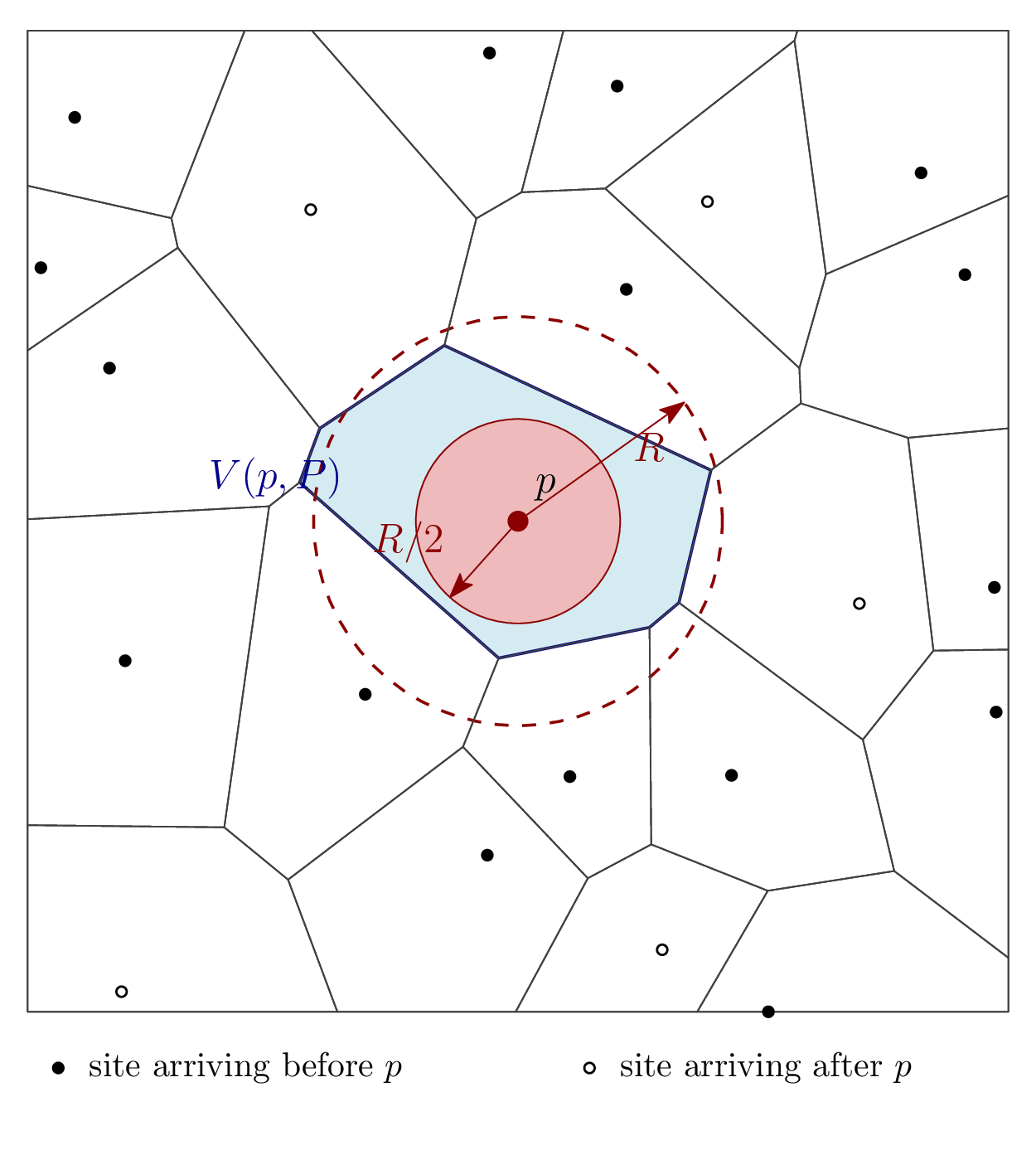
Figure 1: The isolation certificate: the dashed disk $`B(p,R)`$ contains no earlier site. If no later site enters it either, the shaded disk $`B(p,R/2)`$ lies in the final cell of $`p`$.
**Relation to the original strategy.** The rule retains the basic construction of Har-Peled \[[Har26](#X0-h-pvd-26)\]: reserve a final window, accept an arriving site with an empty neighborhood, and bound the chance of a later site entering that neighborhood. Here the target is a sharp approximation to the largest cell, and the window must be specified without knowing the sample count. The tail estimate in [Lemma 3.3](#x1-220013) identifies the sharp area scale; [Lemma 3.5](#x1-230015) supplies enough nearly optimal certificates to use a short window. These are the two inputs to the proof of [Theorem 3.2](#x1-190022).
**Why these parameters fit together.** The intended number of arrivals after $`k`$ is of order $`\lambda /L^2`$. A radius-$`R`$ exclusion disk has area of order $`L/\lambda`$, so their product is $`O(1/L)`$: this is the interference budget in the survival calculation. Meanwhile, $`L^3`$ final isolated sites and a suffix occupying order $`1/L^2`$ of the stream leave order $`L`$ opportunities for selection. The subtraction of $`6\log L`$ in $`\pi \lambda R^2`$ creates this supply of certificates while changing their area by only a vanishing relative amount. The proof below makes both estimates uniform over the relevant realized counts.
#### 3.1.1 The prophet’s payoff
For a unit-intensity Poisson process in $`\mathbb R^2`$, insert a site at the origin and let $`A`$ be its cell area. This is the **typical cell**, rather than the cell containing an independently chosen location.
**Lemma 3.3 (Large-cell tail).** *Let* $`A`$ *be the area of the cell of the inserted origin in a unit-intensity planar Poisson process. For every* $`\delta \in (0,1)`$ *there is* $`c_\delta <\infty`$ *such that, for all* $`a>0`$*,*
```math
e^{-4a}\le {\mathbb{P}}\left[ A\ge a \right] \le c_\delta e^{-4(1-\delta )a}.
```
*Proof:* Write $`r`$ for the largest radius with $`B(0,r)`$ inside the cell and $`r'`$ for the smallest radius with the cell inside $`B(0,r')`$; the inserted origin is the cell’s site, its *nucleus*. Since $`q/2`$ lies on the bisector of $`0`$ and a site $`q`$, the event $`r\ge u`$ is exactly that $`B(0,2u)`$ contains no site, so $`{\mathbb{P}}\left[ r\ge u \right]=e^{-4\pi u^2}`$. As $`A\ge \pi r^2`$, taking $`u=\sqrt {a/\pi }`$ gives the lower bound.
Fix $`\theta >1`$ with $`\theta ^{-2}\ge 1-\delta`$. Hug, Reitzner, and Schneider \[[HRS04](#X0-hrs-lpvc-04), Theorem 1, $`d=k=2`$\] prove that, conditional on $`A\ge a`$, the probability of $`r'/r>\theta`$ tends to zero as $`a\to \infty`$. On $`A\ge a`$ and $`r'/r\le \theta`$, $`a\le \pi r'^2\le \pi \theta ^2r^2`$. Thus, for sufficiently large $`a`$,
```math
\tfrac 12{\mathbb{P}}\left[ A\ge a \right] \le {\mathbb{P}}\left[ r\ge \sqrt {a/(\pi \theta ^2)} \right] =e^{-4a/\theta ^2}.
```
Increase $`c_\delta`$ to cover the remaining values of $`a`$.
Only the qualitative roundness conclusion is needed here. For a self-contained alternative, [Section A](#an-elementary-proof-of-the-largecell-tail) proves the same tail bound by discretizing an empty region. [Figure 2](#two-large-cells-in-one-poisson-sample-of-intensity-107-the-site-with-the-largest-empty-disk-left-and-the-largest-cell-found-right-the-red-disk-has-half-the-radius-of-the-empty-disk-dashed) shows what large cells and their certificates look like in a real sample of intensity $`10^7`$ (generated by tools/gen_large_cell.jl). The displayed cells have areas of about $`5.1`$ and $`6.5`$ mean cell areas, whereas the asymptotic value $`\log \lambda /4`$ of [Theorem 3.2](#x1-190022) is about $`4.0`$ at this intensity; the convergence is slow. The sample count uses a normal approximation to the Poisson count, and both panels show maxima found among the sites with the largest empty disks.
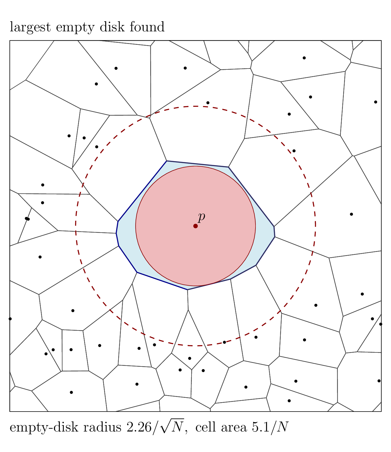 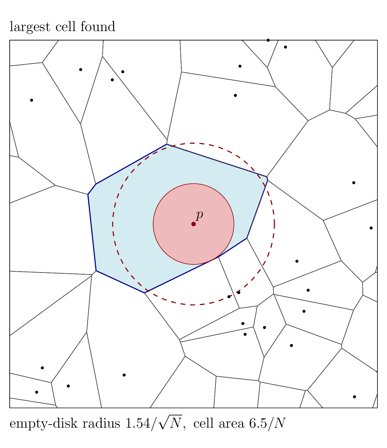
Figure 2: Two large cells in one Poisson sample of intensity $`10^7`$: the site with the largest empty disk (left) and the largest cell found (right). The red disk has half the radius of the empty disk (dashed).
**Lemma 3.4 (Upper bound on the largest cell).** *In the* [*uniform Poisson model*](#x1-180011)*, for every fixed* $`\eta >0`$*, as* $`\lambda \to \infty`$*,*
```math
{\mathbb{P}}\left[ M> \frac {(1+\eta )\log \lambda }{4\lambda } \right]=o(1).
```
*Proof:* *Plan.* First we couple the cell of a site inserted into the torus sample with the typical planar cell of [Lemma 3.3](#x1-220013), using occupied sectors around the inserted site. The tail of that cell then bounds the expected number of sample cells above the threshold, and Markov’s inequality bounds the maximum. Fix $`\delta \in (0,1)`$ with $`(1-\delta )(1+\eta )>1`$.
*From the torus to the plane.* Insert a site at a fixed point of the torus and use Euclidean coordinates centered there; put $`\rho =1/16`$. Since $`2\rho <1/4`$, torus and Euclidean distances agree inside $`B(0,2\rho )`$, and the periodic lift of the torus sample restricted to $`B(0,2\rho )`$ is a planar Poisson process of intensity $`\lambda`$. We may therefore realize a planar Poisson process $`X`$ of intensity $`\lambda`$ that agrees with the lift inside $`B(0,2\rho )`$. Let $`A_{\mathbb T}`$ be the area of the inserted site’s torus cell, and let $`A'`$ be the area of the origin’s cell with respect to $`X\cup \{0\}`$. By scaling, $`A'`$ has the law of $`A/\lambda`$, with $`A`$ as in [Lemma 3.3](#x1-220013).
Partition $`B(0,\rho )`$ into twelve sectors of angle $`\pi /6`$, and let $`E`$ be the event that every sector contains a site of $`X`$. We claim that on $`E`$ both cells lie in $`B(0,\rho )`$ and coincide. Let $`x`$ be any point with $`\|x\|\ge \rho /\sqrt 3`$, and let $`q`$ be a site of $`X`$ in the sector containing the direction of $`x`$. The angle between $`x`$ and $`q`$ is at most $`\pi /6`$, and $`\|q\|<\rho \le \sqrt 3\|x\|`$, so
```math
\|x-q\|^2 \le \|x\|^2-2\|x\|\|q\|\cos (\pi /6)+\|q\|^2 =\|x\|^2-\|q\|\bigl (\sqrt 3\|x\|-\|q\|\bigr )<\|x\|^2.
```
Thus $`x`$ is closer to $`q`$ than to the origin, and the cell of the origin with respect to $`X\cup \{0\}`$ lies in $`B(0,\rho /\sqrt 3)`$. The lifted torus sample contains the same sites inside $`B(0,\rho )`$, so the lifted torus cell lies there as well. Finally, the bisector of the origin and a site outside $`B(0,2\rho )`$ stays outside $`B(0,\rho )`$, so such sites affect neither cell. Both cells are thus determined by the common sites inside $`B(0,2\rho )`$ and agree on $`E`$. A union bound over the sectors gives $`{\mathbb{P}}\left[ E^c \right]\le 12e^{-\lambda \pi \rho ^2/12}`$. With $`c=\pi \rho ^2/12`$ and [Lemma 3.3](#x1-220013),
```math
{\mathbb{P}}\left[ A_{\mathbb T}>a \right] \le {\mathbb{P}}\left[ A'>a \right]+{\mathbb{P}}\left[ E^c \right] \le c_\delta e^{-4(1-\delta )\lambda a}+12e^{-c\lambda }.
```
*From one cell to the largest cell.* The expected number of sample sites whose cell has area greater than $`a`$ is $`\lambda {\mathbb{P}}\left[ A_{\mathbb T}>a \right]`$. Indeed, conditional on $`N=n`$, this expected number is $`n`$ times the probability that a distinguished uniform site has such a cell among $`n-1`$ other uniform sites. Multiply by $`{\mathbb{P}}\left[ N=n \right]`$ and sum over $`n`$; the identity $`n{\mathbb{P}}\left[ N=n \right]=\lambda {\mathbb{P}}\left[ N=n-1 \right]`$ turns the sum into $`\lambda`$ times the probability that a uniformly placed extra site, inserted into an independent Poisson sample of intensity $`\lambda`$, has cell area greater than $`a`$, which is $`{\mathbb{P}}\left[ A_{\mathbb T}>a \right]`$ by translation invariance. Markov’s inequality gives
```math
{\mathbb{P}}\left[ M>a \right] \le c_\delta \lambda e^{-4(1-\delta )\lambda a} +12\lambda e^{-c\lambda }.
```
Set $`a=(1+\eta )L/(4\lambda )`$. The first term is then $`c_\delta \lambda ^{1-(1-\delta )(1+\eta )}=o(1)`$.
#### 3.1.2 Enough isolated sites
Call a sample site $`R`$**-isolated** if no other final site is at distance less than $`R`$ from it. Such a site has $`B(p,R/2)\subseteq V_P(p)`$, by the triangle inequality.
**Lemma 3.5 (Enough isolated sites).** *In the* [*uniform Poisson sampling model*](#x1-180011)*, with* $`L`$ *and* $`R`$ *from* [Eq. (1)](#x1-19001r1) *and* $`\lambda`$ *sufficiently large, the final sample contains at least* $`L^3\)
\(R`$*-isolated sites with probability* $`1-e^{-\Omega (L^4)}`$*.*
*Proof:* *Plan.* Pack disjoint guard disks, each with a much smaller central disk. A guard succeeds when its central disk holds exactly one site and the rest of the guard is empty; that site is then $`R`$-isolated. The guards succeed independently, with expected count of order $`L^4`$, and a Chernoff bound gives $`L^3`$ successes.
Set $`r_0=(\lambda L)^{-1/2}`$ and $`R'=R+2r_0`$. A square grid on the torus supplies $`m=\Omega (R'^{-2})=\Omega (\lambda /L)`$ disjoint disks of radius $`R'`$. For each center $`z`$, require exactly one site in $`B(z,r_0)`$ and no other site in $`B(z,R')`$. The resulting site is $`R`$-isolated, since its radius-$`R`$ disk lies inside $`B(z,R')`$. The events for different centers concern disjoint regions and are therefore independent. Each has probability $`\psi =\lambda \pi r_0^2e^{-\lambda \pi R'^2}`$, the product of the probability $`\lambda \pi r_0^2e^{-\lambda \pi r_0^2}`$ of exactly one site in $`B(z,r_0)`$ and the probability $`e^{-\lambda \pi (R'^2-r_0^2)}`$ of no site in the annulus. Here $`\lambda \pi r_0^2=\pi /L`$, and
```math
\lambda \pi R'^2 =\lambda \pi R^2+4\pi \lambda Rr_0+4\pi \lambda r_0^2 =L-6\log L+O(1),
```
since $`\lambda Rr_0\le 1/\sqrt \pi`$ and $`\lambda r_0^2=1/L`$. Hence
```math
\psi =\frac \pi L\exp \bigl (-L+6\log L-O(1)\bigr ) =\Omega \!\left (\frac {L^5}{\lambda }\right ).
```
The number $`J`$ of successful centers is a sum of $`m`$ independent indicators with mean $`m\psi =\Omega (L^4)`$. For sufficiently large $`\lambda`$ this mean exceeds $`2L^3`$, and a Chernoff bound gives $`{\mathbb{P}}\left[ J
#### 3.1.3 Selection and survival
The proof separates two questions. Whether the rule has an opportunity to stop is decided by the final sample and its order, so we may expose the whole sample and randomize the order. Whether the selected site keeps its certificate must be decided for every stopping history, because the rule may stop at a site that passes its test without being isolated in the final sample; for this question we expose only the count and the observed prefix.
*Proof of (*[Theorem 3.2](#x1-190022)*)* Put $`\Delta =\lambda /L^2`$ and let $`E=\{|N-\lambda |\le \Delta /2\}`$. Poisson concentration gives $`{\mathbb{P}}\left[ E^c \right]\le 2e^{-\Omega (\lambda /L^4)}`$. On $`E`$, for sufficiently large $`\lambda`$,
```math
\Delta /2\le N-k\le 2\Delta , \qquad N\le 2\lambda .
\tag {2}
```
Let $`\tau`$ be the index of the selected site, with $`\tau =\infty`$ if no selection is made. Consider the following four events: (i) $`E^c`$; (ii) the final sample has fewer than $`L^3\) \(R`$-isolated sites; (iii) every $`R`$-isolated site arrives among the first $`k`$ sites; (iv) the rule selects a site $`p_\tau`$ and a later site lies in $`B(p_\tau ,R)`$. If none of them occurs, then some $`R`$-isolated site arrives after position $`k`$ and passes the rule’s test, so a selection $`p_\tau`$ is made. No earlier site lies in $`B(p_\tau ,R)`$, by the test, and no later site does, since (iv) fails. Thus $`p_\tau`$ is $`R`$-isolated in the final sample, its cell contains $`B(p_\tau ,R/2)`$, and
```math
Y\ge \frac {\pi R^2}{4} =\frac {L-6\log L}{4\lambda },
```
which is the claimed bound. It remains to bound the probabilities of the four events. Event (ii) has probability $`e^{-\Omega (L^4)}`$ by [Lemma 3.5](#x1-230015).
**Some isolated site arrives late.** Condition on an unordered final sample satisfying $`E`$ and containing $`I\ge L^3`$ isolated sites. Its order is still uniform, so the positions of these $`I`$ sites form a uniform $`I`$-subset of $`\{1,\ldots ,N\}`$. By [Eq. (2)](#x1-24003r2), the probability that all of them lie in the first $`k`$ positions is at most
```math
(k/N)^I \le e^{-I(N-k)/N} \le \exp \!\left (-L^3\cdot \frac {\Delta /2}{2\lambda }\right ) =e^{-L/4}=\lambda ^{-1/4}.
```
(It is zero if $`I>k`$.) This bounds the probability of (iii) outside (i) and (ii).
**The selected certificate survives.** Condition on $`N=n`$, for an $`n`$ satisfying $`E`$, and on the history $`\mathcal F_\tau`$ through the selection index $`\tau`$. Conditional on $`N=n`$, the ordered locations are independent uniform points. The event $`\tau =i`$ is determined by the first $`i`$ locations, so the remaining $`n-\tau`$ locations are still independent uniform points. Since $`\tau >k`$, [Eq. (2)](#x1-24003r2) and a union bound give
```math
{\mathbb{P}}\left[ \text {a later site lies in }B(p_\tau ,R) \mid N=n,\mathcal F_\tau \right] \le (n-\tau )\pi R^2 \le 2\Delta \pi R^2\le \frac 2L.
```
This bound holds for every stopping history, so averaging over the histories and over $`n`$ bounds the probability of (iv) outside (i) by $`2/L`$.
Altogether, the certificate fails with probability at most
```math
2e^{-\Omega (\lambda /L^4)}+e^{-\Omega (L^4)} +\lambda ^{-1/4}+\frac 2L=O\!\left (\frac 1L\right ),
```
which proves the first assertion. Since $`Y\le M`$, this lower bound and [Lemma 3.4](#x1-220074) imply $`4\lambda M/L\xrightarrow {\mathrm p}1`$ and $`Y/M\xrightarrow {\mathrm p}1`$.
The analysis uses the realized count only for conditioning; the player never learns it. The rule needs no arrival times, no end-of-stream signal, and no selection after the stream ends.
**Finite sizes.** The theorem is asymptotic, and the asymptotics are slow. The radius $`R`$ in [Eq. (1)](#x1-19001r1) is undefined until $`L>6\log L`$, that is, $`\lambda`$ beyond about $`2\times 10^7`$, and the failure probability decays only like $`1/\log \lambda`$. [Table 3](#simulation-of-the-finitesize-variant-of-the-rule-with-3-l-in-place-of-6-l-on-the-unit-torus-y-is-the-payoff-and-m-the-largest-final-cell-both-computed-exactly) reports a simulation (tools/sim_poisson_rule.jl) of the natural finite-size variant with $`3\log L`$ in place of $`6\log L`$, for which the expected number of final $`R`$-isolated sites is about $`L^3`$, the amount the proof uses. Two effects dominate at these sizes. First, the largest cell is still $`1.7`$ to $`2`$ times its asymptotic value $`\log \lambda /(4\lambda )`$, while the certified area $`\pi R^2/4`$ is at most a quarter of it; the selected cell is larger than its certificate, which is why $`Y/M`$ exceeds the certified fraction. Second, for $`\lambda \le 10^4`$ the suffix of about $`\lambda /\log ^2\lambda`$ intended arrivals is comparable to or smaller than the fluctuation $`\sqrt \lambda`$ of the hidden count, so the stream often ends before position $`k`$ and nothing is selected. This is the price of not knowing $`N`$; the no-selection rate falls to $`2\%`$ at $`\lambda =10^5`$ and to $`0\%`$ at $`10^6`$. A selection is made and its certificate survives in $`69\%`$, $`83\%`$, $`98\%`$, and $`100\%`$ of all trials at the four intensities, so conditional on a selection the certificate survives in about $`95\%`$ of the trials at the two smaller intensities and in all trials at the two larger ones.
| $`\lambda`$ | trials | mean $`Y/M`$ | median $`Y/M`$ | $`{\mathbb{P}}\left[ Y\ge M/2 \right]`$ | $`{\mathbb{P}}\left[ \text {no selection} \right]`$ | mean $`4\lambda M/\log \lambda`$ |
|----|----|----|----|----|----|----|
| $`10^3`$ | $`400`$ | $`0.30`$ | $`0.32`$ | $`0.18`$ | $`0.27`$ | $`2.06`$ |
| $`10^4`$ | $`200`$ | $`0.39`$ | $`0.40`$ | $`0.28`$ | $`0.13`$ | $`1.88`$ |
| $`10^5`$ | $`50`$ | $`0.46`$ | $`0.43`$ | $`0.30`$ | $`0.02`$ | $`1.76`$ |
| $`10^6`$ | $`10`$ | $`0.48`$ | $`0.44`$ | $`0.30`$ | $`0.00`$ | $`1.68`$ |
Table 3: Simulation of the finite-size variant of the rule, with $`3\log L`$ in place of $`6\log L`$, on the unit torus; $`Y`$ is the payoff and $`M`$ the largest final cell, both computed exactly.
### 3.2 A factor-two barrier for smooth densities
We now return to a known, fixed sample size. For a smooth density the answer is very different from the uniform case: a density may place equal mass $`1/m`$ in tiny bumps of radius $`\epsilon s`$ around the $`m`$ points of a regular grid of spacing $`s`$. Call the set of sites falling into one bump its *bin*. A site alone in its bin gets a full grid cell; every site sharing its bin gets at most half as much ([Figure 3](#the-bumpgrid-density-with-the-bump-radius-exaggerated-a-singleton-bin-shaded-cell-owns-essentially-its-whole-grid-square-the-sites-of-a-bin-with-two-or-three-sites-split-theirs)). The player has trouble recognizing which early arrivals will remain alone.
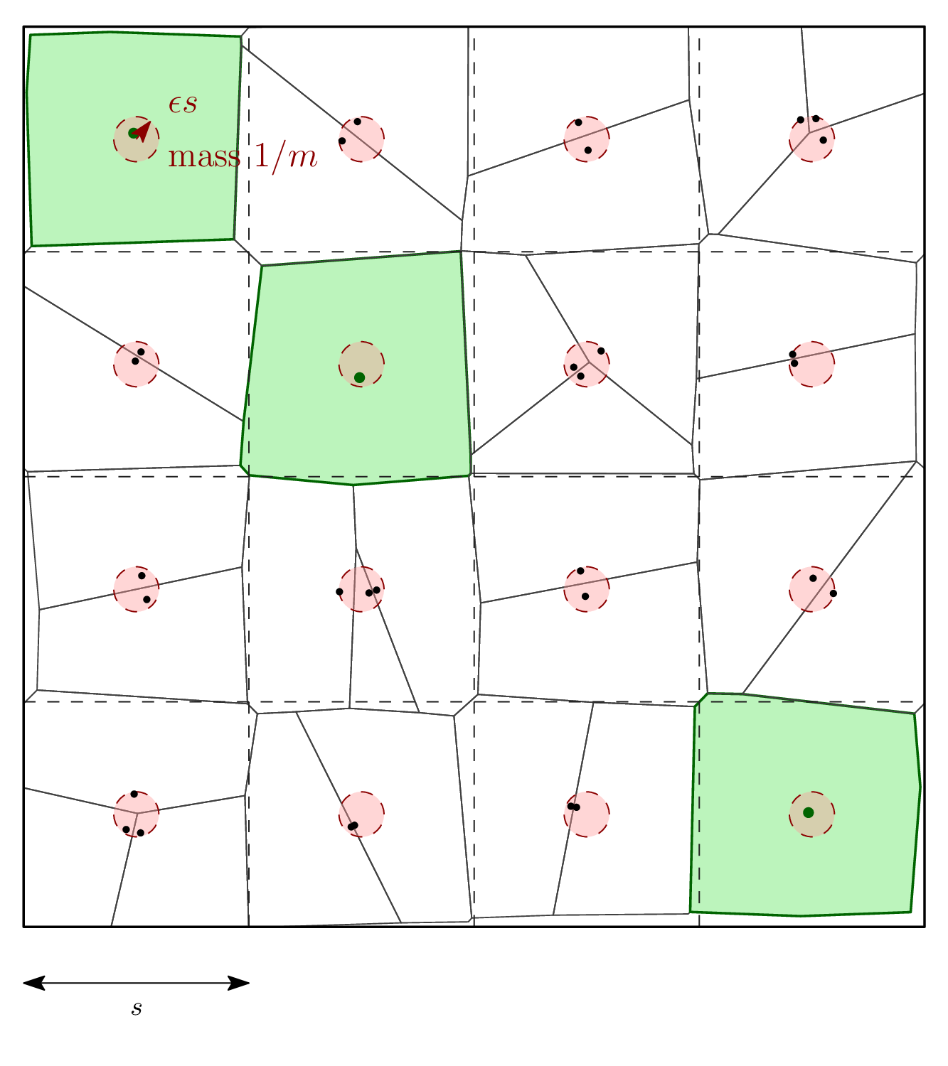
Figure 3: The bump-grid density, with the bump radius exaggerated. A singleton bin (shaded cell) owns essentially its whole grid square; the sites of a bin with two or three sites split theirs.
**Theorem 3.6 (Factor-two barrier).** *In the* [*smooth random-sample setting*](#x1-160015)*, on the circle or in the plane, there is a sequence of sample sizes* $`n\to \infty`$ *and known laws* $`F_n`$ *with* $`C^\infty`$ *densities having the following property. For every fixed* $`B\geq 0`$*, every online strategy selecting at most* $`(\log n)^B`$ *of the* $`n`$ *independent sites satisfies, for each fixed* $`1\leq \alpha <2`$*,*
```math
{\mathbb{P}}\left[ Y\geq M/\alpha \right] =O_B\!\left (\frac {\log \log n}{\sqrt {\log n}}\right )=o(1), \qquad {\mathbb{E}}\left[ Y \right]\leq \bigl (1/2+o(1)\bigr ){\mathbb{E}}\left[ M \right].
```
*Here* $`Y`$ *is the largest final cell among the selected sites. The bounds hold even when the strategy knows the density. The density changes with* $`n`$ *and may vanish.*
The proof reduces the game to a balls-in-bins selection problem: bumps are bins, and a singleton bin owns a full grid square. The sample size is tuned so that, with high probability, every bin is occupied and about $`\sqrt {\log m}`$ bins are singletons. The singleton-selection lemma below makes selecting one of those singletons unlikely, while the geometric lemma that follows bounds every other cell by about half a grid square. For the expectation bound, empty bins are temporarily filled and the extra area is charged to the number of temporary sites.
Problem 3.7 (Singleton selection). There are $`m\ge 2`$ known bins and $`n`$ independent balls, each assigned to a uniformly random bin. The player knows $`m,n`$ and a budget $`b`$, and observes each ball’s bin upon arrival. It may select at most $`b`$ balls irrevocably upon arrival, with no recall. Success means that some selected ball is the only final ball in its bin. The player may also observe auxiliary marks whose conditional distribution, given that ball’s bin, is independent of all other balls and marks. (In the reduction, the mark is the exact location of a site inside its bump.)
**Lemma 3.8 (Singleton selection).** *In the* [*singleton-selection problem*](#x1-280047)*, put* $`q=1-1/m`$*. For every integer* $`0\le f\le n`$ *and every strategy,*
```math
{\mathbb{P}}\left[ \text {a selected ball is a final singleton} \right] \le bq^f+fq^{n-1}.
```
*Proof:* Split the arrivals into a prefix of length $`n-f`$ and a suffix of length $`f`$; the first term accounts for prefix selections, which must survive the suffix, and the second for suffix balls, which are rarely final singletons at all. Each selection among the first $`n-f`$ arrivals has conditional success probability at most $`q^f`$: at least $`f`$ independent future balls must avoid its bin. Sum over the at most $`b`$ selections. Each of the last $`f`$ balls has unconditional singleton probability $`q^{n-1}`$. A union bound over those balls gives the second term. The auxiliary marks give no information about future bin labels.
The following lemma makes the geometry of the reduction quantitative.
**Lemma 3.9 (Perturbed grid cells).** *In dimension* $`d\in \{1,2\}`$*, let* $`D=\mathbb T^d`$ *and let* $`\mu _D`$ *be length or area. Place* $`m=h^d`$ *centers on the regular grid in* $`D`$*, with spacing* $`s=1/h`$ *for an integer* $`h\ge 4`$*. For each center* $`z`$*, its bin consists of one or more distinct sites within distance* $`\epsilon s`$ *of* $`z`$*, where* $`0<\epsilon \le 1/100`$*. Let* $`U_z`$ *be the union of the cells of that bin’s sites in the Voronoi diagram of all the bins’ sites together. There is an absolute constant* $`c`$ *such that*
```math
\frac {1-c\epsilon }{m}\le \mu _D(U_z) \le \frac {1+c\epsilon }{m}.
```
*A singleton bin therefore gives a cell of this size. If a bin contains at least two sites, each of its cells has measure at most* $`(1/2+c\epsilon )/m`$*.*
*Proof:* *Plan.* Trap the territory of one bin between a slightly contracted and a slightly expanded grid box; this bounds its measure. To bound one cell in a bin with several sites, compare its site with one other site of the bin: their bisector passes close to the center, so central symmetry bounds the cell by about half the box.
Translate the center under consideration to $`0`$ and work with lifts in $`\mathbb R^d`$; there $`\mu _D`$ denotes Euclidean length or area, and $`e_i`$ is the $`i`$th standard coordinate vector. Since $`h\ge 4`$, all points below lie within one coordinate neighborhood of the torus, where Euclidean and torus distances agree. Let $`W=[-s/2,s/2]^d`$ be the grid cell of $`0`$. Two facts are used repeatedly. First, for any location $`x`$, the distance from $`x`$ to the nearest site of the bin at a center $`z`$ differs from $`\|x-z\|`$ by at most $`\epsilon s`$. Second, for any point $`x`$ and the center $`z'=\operatorname {sign}(x_i)\,se_i`$, with $`\operatorname {sign}(0)=1`$,
```math
\|x-z'\|^2-\|x\|^2=s^2-2s|x_i|.
\tag {3}
```
**Outer box.** Let $`x`$ be the lift closest to $`0`$ of a location in $`U_0`$. Every location has a grid center within distance $`\sqrt d\,s/2`$, hence a site within distance $`\sqrt d\,s/2+\epsilon s`$. Some site of the bin at $`0`$ owns $`x`$ and is therefore at least as close to $`x`$, so $`\|x\|\le \sqrt d\,s/2+2\epsilon s **Inner box.** Let $`x`$ satisfy $`|x_i|\le s/2-4\epsilon s`$ for every $`i`$. For a center $`z=s(z_1,\ldots ,z_d)\ne 0`$ with integer coordinates,
```math
\|x-z\|^2-\|x\|^2 =\sum _i\bigl (s^2z_i^2-2sx_iz_i\bigr ) \ge \sum _i|z_i|\,s\bigl (s-2|x_i|\bigr ),
```
using $`z_i^2\ge |z_i|`$ and $`|x_i|\le s/2`$. Since $`s-2|x_i|\ge 8\epsilon s`$ for every $`i`$ and $`\sum _i|z_i|\ge 1`$, the right side is at least $`8\epsilon s^2`$. Apply this to a grid center $`z'\neq 0`$ nearest to $`x`$, which satisfies $`\|x-z'\|\le \|x\|+s<2s`$: dividing by $`\|x-z'\|+\|x\|\le 3s`$ gives $`\|x-z'\|-\|x\|\ge 8\epsilon s/3>2\epsilon s`$, and every other center is at least as far from $`x`$ as $`z'`$. Hence every site of the bin at $`0`$ is strictly closer to $`x`$ than every site of any other bin, so $`x\in U_0`$. Thus $`[-s/2+4\epsilon s,s/2-4\epsilon s]^d\subseteq U_0`$.
The two boxes have measures $`s^d(1-O(\epsilon ))`$ and $`s^d(1+O(\epsilon ))`$. This proves the first assertion and shows $`\mu _D(U_0\mathbin \triangle W)=O(\epsilon /m)`$.
**Two sites in one bin.** Let $`p,p'`$ be two sites of the bin at $`0`$. The cell of $`p`$ lies in the halfspace $`H=\{x:\|x-p\|\le \|x-p'\|\}`$, whose boundary passes through the midpoint of $`p`$ and $`p'`$, at distance at most $`\epsilon s`$ from $`0`$. Let $`H'`$ be the translate of $`H`$ whose boundary passes through $`0`$. By the central symmetry of $`W`$, $`\mu _D(H'\cap W)=\mu _D(W)/2`$, and $`H\setminus H'`$ is a strip of width at most $`\epsilon s`$, meeting $`W`$ in measure at most $`\epsilon s\,(\sqrt d\,s)^{d-1}`$. Therefore the cell of $`p`$ has measure at most $`\mu _D(H\cap W)+\mu _D(U_0\setminus W)\le (1/2+c\epsilon )/m`$.
*Proof of (*[Theorem 3.6](#x1-280026)*)* Let $`m\to \infty`$, put $`\Lambda =\log m`$, and take
```math
n=\left \lfloor m\left (\Lambda +\tfrac 12\log \Lambda \right )\right \rfloor .
```
On the circle use $`m`$ equally spaced centers. On the torus take $`m`$ to be a square and use a regular square grid. Write $`s`$ for the grid spacing, and let $`\epsilon _m=m^{-3}`$. Give each center probability $`1/m`$, distributed by a smooth bump inside distance $`\epsilon _m s`$ of that center. Each sampled point is distinct almost surely. Its center label is an independent uniform bin label.
**Occupancies.** Let $`Z_0`$ and $`Z_1`$ count the empty and singleton bins after all $`n`$ draws. Directly,
```math
{\mathbb{E}}\left[ Z_0 \right]=m(1-1/m)^n\sim \Lambda ^{-1/2}, \qquad {\mathbb{E}}\left[ Z_1 \right]=n(1-1/m)^{n-1}\sim \sqrt \Lambda .
```
More generally, if $`Z_1(t)`$ counts singleton bins after $`t`$ draws,
```math
{\mathbb{E}}\left[ Z_1(t)(Z_1(t)-1) \right] =(1-1/m)t(t-1)(1-2/m)^{t-2}.
```
For $`t=n+o(m)`$, expansion of these expressions gives $`{\mathbb{E}}\left[ Z_1(t) \right]\sim \sqrt \Lambda`$ and $`{\mathbb{V}}\left[ Z_1(t) \right]=O(\sqrt \Lambda )`$. Markov’s and Chebyshev’s inequalities therefore give
```math
{\mathbb{P}}\left[ Z_0>0 \right]+{\mathbb{P}}\left[ Z_1=0 \right]=O(\Lambda ^{-1/2}).
```
In particular, with high probability all bins are occupied and there is a singleton.
**Geometry.** When all bins are occupied, [Lemma 3.9](#x1-280109) gives cell measure $`(1\pm c\epsilon _m)/m`$ for a singleton and at most $`(1/2+c\epsilon _m)/m`$ for every site that shares its bin.
To bound $`Y`$ and $`M`$ on every outcome, including those with empty bins, insert a temporary site at each empty center. In the enlarged configuration all bins are occupied, so the lemma applies: each temporary site is a singleton with cell measure at most $`(1+c\epsilon _m)/m`$, and each original site has the measure stated above. Removing the temporary sites enlarges an original site’s cell only by parts of their former cells, whose total measure is at most $`(1+c\epsilon _m)Z_0/m`$. Writing $`I`$ for the indicator that some selected site is a final singleton, we obtain
```math
Y\leq \frac {1/2+c\epsilon _m +(1/2)I+(1+c\epsilon _m)Z_0}{m}, \qquad M\leq \frac {(1+c\epsilon _m)(1+Z_0)}{m}.
```
When every bin is occupied and some bin is a singleton, which holds with high probability by the occupancy estimates, $`M\geq (1-c\epsilon _m)/m`$; together with the upper bound and $`{\mathbb{E}}\left[ Z_0 \right]=o(1)`$, this gives $`{\mathbb{E}}\left[ M \right]=(1+o(1))/m`$.
**Online selection.** Apply [Lemma 3.8](#x1-280068) with $`f=\lceil (B+2)m\log \Lambda \rceil`$. Since $`(1-1/m)^{n-1}\sim 1/(m\sqrt \Lambda )`$ and $`\log n\sim \Lambda`$,
```math
{\mathbb{P}}\left[ I=1 \right] \leq (\log n)^B(1-1/m)^f +f(1-1/m)^{n-1} =O_B\!\left (\frac {\log \Lambda }{\sqrt \Lambda }\right ).
```
If every bin is occupied and a singleton exists, approximation better than any fixed $`\alpha <2`$ requires selecting a singleton, for sufficiently large $`m`$. Adding the occupancy failure probability proves the success bound. Taking expectations in the bound for $`Y`$ proves the expected-payoff assertion.
#### 3.2.1 A matching strategy for this family
**Proposition 3.10 (Matching strategy).** *In the* [*smooth random-sample setting*](#x1-160015)*, on the circle or in the plane, one selection on the bump-grid family constructed in the proof of* [Theorem 3.6](#x1-280026) *obtains* $`Y\geq M/(2+o(1))`$ *with probability* $`1-O((\log n)^{-1/4})`$*, and* $`{\mathbb{E}}\left[ Y \right]\geq (1/2-o(1)){\mathbb{E}}\left[ M \right]`$*.*
*Proof:* *Plan.* Near the end, many bins still contain exactly one site. Accept the first later arrival into one of them; the short suffix makes a third arrival into that bin unlikely, and the two final sites then split about one grid cell equally.
Use $`m`$, $`n`$, $`\Lambda =\log m`$, and $`\epsilon _m=m^{-3}`$ from the proof of [Theorem 3.6](#x1-280026), and put $`f=\lfloor m/\Lambda ^{1/4}\rfloor`$. After the first $`n-f`$ sites, record the set $`\mathcal S`$ of bins containing exactly one site. Select the first subsequent arrival in a bin of $`\mathcal S`$. If none occurs earlier, select the last site.
The moment calculation in [Theorem 3.6](#x1-280026) shows that $`|\mathcal S|\geq \sqrt \Lambda /2`$ except with probability $`O(\Lambda ^{-1/2})`$. Conditional on this prefix, the probability that all $`f`$ remaining sites avoid $`\mathcal S`$ is at most
```math
(1-|\mathcal S|/m)^f\leq \exp (-\Omega (\Lambda ^{1/4})).
```
If a suffix arrival hits $`\mathcal S`$, the rule selects the first such arrival, and its bin then contains exactly two sites. Conditional on this stopping history, the probability of a further arrival in that bin is at most $`f/m=O(\Lambda ^{-1/4})`$. Thus its final occupancy is two with high probability.
If all bins are occupied, the two cells of a two-site bin together have measure $`(1+O(\epsilon _m))/m`$, and each has measure at most $`(1/2+O(\epsilon _m))/m`$. Each therefore has measure $`(1/2+O(\epsilon _m))/m`$. Since also $`M\leq (1+O(\epsilon _m))/m`$, the probability assertion follows. Nonnegativity of the payoff and $`{\mathbb{E}}\left[ M \right]=(1+o(1))/m`$ give the expectation bound.
The matching statement concerns this bump-grid family.
### 3.3 A constant approximation in one dimension
On the circle, knowledge of the sampling distribution suffices for a constant approximation. The strategy observes the first half of the arrivals. It then either runs an ordinary secretary rule, or monitors disjoint intervals with different activation times. All intervals and activation times are computed from the distribution before any arrival.
**Theorem 3.11 (Known laws on the circle).** *In the* [*random-sample setting*](#x1-150063) *on the circle, there are absolute constants* $`c_1,c_2>0`$ *such that, for every* $`n\geq 1`$ *and every sampling measure* $`F`$*, a one-choice strategy satisfies*
```math
{\mathbb{E}}\left[ Y \right]\geq \frac {{\mathbb{E}}\left[ M \right]}{7000},\qquad {\mathbb{P}}\left[ Y\geq c_1M \right]\geq c_2.
```
*It selects only after the first* $`\lfloor n/2\rfloor`$ *arrivals. The constants are independent of* $`F`$ *and* $`n`$*.*
The same argument applies to a non-atomic law on the interval $`[0,1]`$ with cells clipped to the interval; only the two boundary gaps need separate bookkeeping, which costs a constant factor. We omit the details.
**A geometric scale determined by the distribution.** Equal probability intervals are not suitable units of payoff: the reward is length, and an interval of small probability may be long. We instead partition into equal *geometric* intervals and use their probabilities only to estimate emptiness. In the next lemma, $`Q_\ell`$ is the expected number of empty intervals at level $`\ell`$. The first level where this expectation reaches $`1/2`$ provides a length $`a`$ that controls the prophet’s expected payoff. Minimality of the level is crucial: it bounds the chance of a much longer empty gap, even when $`F`$ concentrates its mass very unevenly.
**Lemma 3.12 (Gap scale).** *In the* [*random-sample setting*](#x1-150063) *on the circle, let* $`n\geq 2`$*, partition the circle into* $`2^\ell`$ *equal arcs* $`\mathcal D_\ell`$*, and put*
```math
Q_\ell =\sum _{B\in \mathcal D_\ell }(1-F(B))^n.
```
*Let* $`\ell _0`$ *be the first level with* $`Q_{\ell _0}\geq 1/2`$*, and put* $`a=2^{-\ell _0}`$*. For* $`n`$ *independent samples from* $`F`$*, let* $`G`$ *be the largest gap between consecutive sites. Then*
```math
{\mathbb{P}}\left[ G>2^{k+2}a \right]\leq 2^{-2^k},\qquad k=0,1,\ldots , \qquad \text {and}\qquad {\mathbb{E}}\left[ G \right]\leq 12a.
```
*In particular, the expected largest cell satisfies* $`{\mathbb{E}}\left[ M \right]\leq 12a`$*.*
*Proof:* The level exists: Bernoulli’s inequality gives $`Q_\ell \geq 2^\ell -n`$, whereas $`Q_0=0`$. If $`B`$ has dyadic children $`B_1,B_2`$, then
```math
(1-F(B))^n \leq (1-F(B_1))^n(1-F(B_2))^n.
```
Summing over parents gives $`Q_{\ell -1}\leq Q_\ell ^2`$, because a sum of products of nonnegative terms is at most the square of their sum. Since $`Q_{\ell _0-1}<1/2`$, iterating gives $`Q_{\ell _0-1-k}\leq 2^{-2^k}`$ whenever this level exists. The arcs of level $`\ell _0-1-k`$ have length $`2^{k+1}a`$, and a gap longer than $`2^{k+2}a`$ contains one of them entirely. Thus the probability of such a gap is at most the expected number of empty arcs at that level, namely $`Q_{\ell _0-1-k}`$. If the level does not exist, then $`2^{k+2}a>1`$ and the event is empty.
Integrating over these dyadic ranges gives
```math
{\mathbb{E}}\left[ G \right]\leq 4a+4a\sum _{k\geq 0}2^k2^{-2^k} \leq 4a+4a\sum _{i\geq 1}i2^{-i}=12a.
```
Finally, every cell is half the sum of its two incident gaps, so $`M\leq G`$.
**Turning the scale into an online choice.** The proof of [Theorem 3.11](#x1-3600111) seeks a cell of length $`a/4`$ with constant probability. Within each arc of length $`a`$, its less probable half offers room for such a cell. If one of these halves has probability at most $`1/n`$, an ordinary secretary rule, scoring sites by their distance to the half’s midpoint, finds the site nearest that midpoint ([Lemma 3.13](#x1-3900113)). Otherwise, each half is paired with a short adjacent interval of probability $`1/n`$, where the selected site should land. Each pair receives its own activation time, chosen so that the expected number of later hits to it is at most a constant, and a second-moment calculation shows that enough of these opportunities remain after paying for their different waiting times ([Lemma 3.14](#x1-3900514)). [Figure 4](#one-monitored-pair-jj-is-the-half-of-bj-with-the-smaller-mass-and-wj-the-adjacent-interval-of-mass-1n-if-p-wj-is-the-only-final-site-in-hj-the-final-cell-of-p-has-length-at-least-a4), placed after the definitions, shows one monitored pair: the empty half $`J_j`$ supplies the guaranteed length, and $`W_j`$ is the interval in which the selected site should land.
**Standing notation.** Fix $`F`$ and $`n\geq 4`$. Use the scale $`a`$ and the partition $`\mathcal D_{\ell _0}`$ from [Lemma 3.12](#x1-3700112). Write its arcs as $`B_j`$, with
```math
\beta _j=F(B_j),\qquad q_j=(1-\beta _j)^n, \qquad \sum _j q_j\geq \frac 12.
```
Split each $`B_j`$ into its two equal halves. Let $`J_j`$ be a half of smaller probability mass, breaking ties deterministically, and put $`r_j=F(J_j)\leq \beta _j/2`$. Its length is $`a/2`$.
**Lemma 3.13 (A half interval of small mass).** *In the* [*circle random-sample setting*](#x1-150063) *with the standing notation above, if* $`r_j\leq 1/n`$ *for some* $`j`$*, then there is a one-choice strategy that selects only after the first* $`\lfloor n/2\rfloor`$ *arrivals and has* $`{\mathbb{P}}\left[ Y\geq a/4 \right]\geq 1/16`$*.*
*Proof:* Fix such a $`j`$ and the midpoint $`z`$ of $`J_j`$. Ignore the first $`m=\lfloor n/2\rfloor`$ arrivals and use the secretary rule to select the closest site to $`z`$: accept the first later site that is closer to $`z`$ than every site among the first $`m`$. Conditional on any final set, the order is uniform, so this rule selects the closest site with probability
```math
\frac {m}{n}\sum _{t=m+1}^n\frac 1{t-1} \ge \frac {m(n-m)}{n(n-1)}\ge \frac 14.
```
The event that $`J_j`$ contains no final site has probability
```math
(1-r_j)^n\geq (1-1/n)^n\geq \frac 14.
```
On this event the closest site to $`z`$ owns at least half of $`J_j`$: the owners of points inside an empty interval are its two neighboring sites, and the owner of the midpoint receives at least half the interval. Thus, for every final set with no site in $`J_j`$, the secretary rule succeeds with conditional probability at least $`1/4`$, and such sets have probability at least $`1/4`$; so $`{\mathbb{P}}\left[ Y\geq a/4 \right]\geq 1/16`$.
**Lemma 3.14 (Activation rule).** *Under the same standing assumptions, if* $`r_j>1/n`$ *for every* $`j`$*, then there is a one-choice strategy that selects only after the first* $`\lfloor n/2\rfloor`$ *arrivals and has*
```math
{\mathbb{P}}\left[ Y\geq a/4 \right]\geq \delta :=\frac {1}{48e}.
```
*Proof:* *The rule.* The other half of $`B_j`$ has mass at least $`r_j>1/n`$. Choose within that half an interval $`W_j`$ adjacent to $`J_j`$ with $`F(W_j)=1/n`$; non-atomicity guarantees its existence. Define
```math
H_j=J_j\cup W_j,\qquad s_j=F(H_j)=r_j+1/n,\qquad f_j=\lfloor 1/s_j\rfloor .
```
The $`H_j`$ are disjoint, since each lies in its own $`B_j`$. Moreover, $`2/n
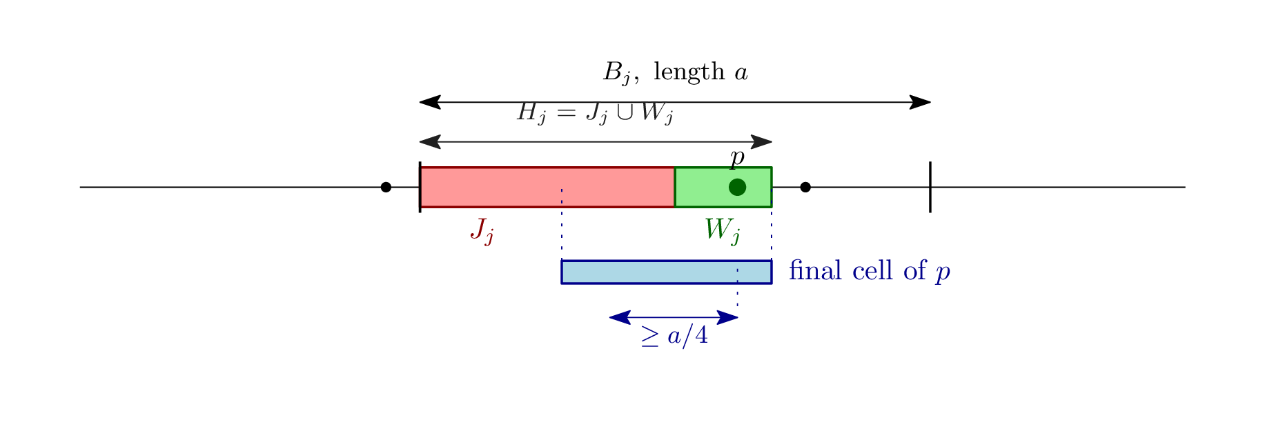
Figure 4: One monitored pair: $`J_j`$ is the half of $`B_j`$ with the smaller mass and $`W_j`$ the adjacent interval of mass $`1/n`$. If $`p\in W_j`$ is the only final site in $`H_j`$, the final cell of $`p`$ has length at least $`a/4`$.
At arrival $`t`$, select the current site if, for some $`j`$, it belongs to $`W_j`$, no earlier site belongs to $`H_j`$, and $`t>n-f_j`$. Call this a *trigger* for $`H_j`$, and stop at the first trigger. If none occurs, select the last site. This is an online rule, and it selects only in the last half of the sequence.
*A trigger survives with constant probability.* Condition on a history in which $`H_j`$ triggers at time $`t>n-f_j`$. The $`n-t\le f_j-1`$ future sites are independent of the history, so the probability that none of them falls in $`H_j`$ is at least
```math
(1-s_j)^{f_j-1} \geq (1-s_j)^{1/s_j-1}\geq e^{-1}.
```
On this event the selected site is the only final site in $`H_j`$. It lies in $`W_j`$ and borders an empty interval that contains $`J_j`$, so its final cell has length at least $`a/4`$.
*A trigger occurs with constant probability.* Let $`E_j`$ be the event that $`H_j`$ contains exactly one final site, that this site lies in $`W_j`$, and that it arrives in the last $`f_j`$ positions. For each of the $`n`$ sites, the probability of lying in $`W_j`$ is $`F(W_j)=1/n`$, the probability that the other $`n-1`$ sites avoid $`H_j`$ is $`(1-s_j)^{n-1}`$, and the probability of arriving in the last $`f_j`$ positions is $`f_j/n`$; summing over the site gives
```math
b_j:={\mathbb{P}}\left[ E_j \right]=\frac {f_j}{n}(1-s_j)^{n-1}.
```
We compare $`b_j`$ with the empty-arc probability $`q_j`$ because $`\sum _jq_j\geq 1/2`$: the gain from using the less probable half must compensate for the short activation window. We claim that $`b_j\geq q_j/16`$. If $`\beta _j=1`$ then $`q_j=0`$ and there is nothing to prove, so assume $`\beta _j<1`$. The claim follows by multiplying the three estimates
```math
\frac {f_j}{n} \geq \frac {1}{2ns_j} \geq \frac {1}{2+n\beta _j},
\tag {4}
```
```math
(1-s_j)^{n-1} \geq \tfrac 18(1-\beta _j/2)^n,
\tag {5}
```
```math
(1-\beta _j/2)^n \geq (1+n\beta _j/2)(1-\beta _j)^n.
\tag {6}
```
For [Eq. (4)](#x1-39010r4), use $`f_j=\lfloor 1/s_j\rfloor \geq 1/(2s_j)`$ (as $`1/s_j\geq 1`$) and $`ns_j=nr_j+1\leq n\beta _j/2+1`$. For [Eq. (5)](#x1-39011r5), write $`1-s_j=(1-r_j)(1-1/(n(1-r_j)))`$ and use $`r_j\leq 1/2`$:
```math
(1-s_j)^{n-1} \geq (1-r_j)^{n-1}\left (1-\frac 2n\right )^{n-1} \geq \tfrac 18(1-r_j)^n \geq \tfrac 18(1-\beta _j/2)^n,
```
since $`(1-2/n)^{n-1}`$ increases with $`n`$ and equals $`1/8`$ at $`n=4`$. For [Eq. (6)](#x1-39012r6), Bernoulli’s inequality gives
```math
\left (\frac {1-\beta _j/2}{1-\beta _j}\right )^n =\left (1+\frac {\beta _j}{2(1-\beta _j)}\right )^n \geq 1+\frac {n\beta _j}2.
```
Put $`Z=\sum _j\mathbf 1_{E_j}`$ and $`\nu ={\mathbb{E}}\left[ Z \right]`$, so $`\nu \geq \tfrac 1{16}\sum _jq_j\geq 1/32`$. For $`i\ne j`$, counting the possible ordered positions of the two unique arrivals gives
```math
{\mathbb{P}}\left[ E_i\cap E_j \right] =\frac {f_if_j-\min \{f_i,f_j\}}{n^2} (1-s_i-s_j)^{n-2} \leq 16b_ib_j,
```
because $`1-s_i-s_j\leq (1-s_i)(1-s_j)`$ and $`(1-s_i)(1-s_j)\geq 1/16`$. Hence, as $`\nu /(1+16\nu )`$ increases with $`\nu`$,
```math
{\mathbb{E}}\left[ Z^2 \right]\leq \nu +16\nu ^2, \qquad {\mathbb{P}}\left[ Z>0 \right]\geq \frac {\nu ^2}{{\mathbb{E}}\left[ Z^2 \right]} \geq \frac {\nu }{1+16\nu } \geq \frac {1}{48}.
```
*Conclusion.* Whenever $`Z>0`$, some $`E_j`$ occurs, and the unique site of $`H_j`$ triggers at its arrival unless the rule has already stopped at an earlier trigger. Either way a trigger occurs, so a trigger occurs with probability at least $`{\mathbb{P}}\left[ Z>0 \right]\geq 1/48`$. Separately, conditional on any history at the first trigger, the region $`H_j`$ of that trigger receives no later site with probability at least $`e^{-1}`$. Averaging this over the triggering histories gives $`{\mathbb{P}}\left[ Y\geq a/4 \right]\geq e^{-1}/48=\delta`$.
*Proof of (*[Theorem 3.11](#x1-3600111)*)* For $`n\leq 3`$, select the last arrival: by symmetry its expected cell length is $`1/n\geq {\mathbb{E}}\left[ M \right]/3`$, and it is an optimal site with probability at least $`1/n`$. For $`n\geq 4`$, use the standing notation above. If some $`r_j\le 1/n`$, apply [Lemma 3.13](#x1-3900113); otherwise apply [Lemma 3.14](#x1-3900514). In both cases $`{\mathbb{P}}\left[ Y\geq a/4 \right]\geq \delta`$, since $`1/16\ge \delta`$. Together with $`{\mathbb{E}}\left[ M \right]\leq 12a`$ from [Lemma 3.12](#x1-3700112), this yields $`{\mathbb{E}}\left[ Y \right]\geq (\delta /48){\mathbb{E}}\left[ M \right]`$, and $`48/\delta =2304e<7000`$. Finally, the tail in [Lemma 3.12](#x1-3700112) gives an absolute constant $`c`$ with $`{\mathbb{P}}\left[ M>ca \right]<\delta /2`$. On the event $`\{Y\geq a/4\}\cap \{M\le ca\}`$, which has probability at least $`\delta /2`$, we have $`Y\geq M/(4c)`$.
The strategy avoids committing to one sample cell. In the second case, it monitors all the disjoint intervals simultaneously. A region of large probability mass is activated later, when its remaining interference is bounded. Splitting $`B_j`$ in half increases its chance of remaining empty enough to pay for the shorter activation window.
## 4 Random arrival and missing vertices
In the [random-arrival setting](#x1-150042), the sites are fixed and unknown; only their order is random. [Theorem 4.3](#x1-430013) shows that a single choice guarantees an $`O(\log n)`$ approximation. By [Theorem 4.4](#x1-440014), even $`\sqrt n`$ choices can lose a factor $`\Omega (\log n/\log \log n)`$ in expected payoff. More generally, constant expected competitiveness in the plane requires a linear selection budget ([Corollary 4.6](#x1-470016)). The missing-vertex game then isolates the underlying information problem and admits an exact optimal stopping rule ([Lemma 4.9](#x1-510019)).
### 4.1 A logarithmic approximation
**From a current cell to its final owner.** Write $`V_{P_t}(p)`$ for the *current cell* of $`p\in P_t`$ after $`t`$ arrivals; the final cell $`V_P(p)`$ is contained in it. A large current cell need not remain large. Instead of trying to preserve its entire area, the strategy samples a location inside a large part of it and tries to select that location’s final owner. [Lemma 4.1](#x1-420021) supplies a stopping time at which a large current cell is available with constant probability. [Lemma 4.2](#x1-420072) then bounds the number of final cells that can divide a suitable triangle inside it by $`O(\log n)`$. Sampling a location favors owners receiving more of this area. Finally, that location turns the search for an unseen owner into a secretary problem with a fixed score: distance to the location. This separates the argument into a stopping calculation, a geometric bound on fragmentation, and a standard selection step.
Break all ties by a fixed ordering of the sites, independent of their arrival order. For a nonempty set $`Q`$, let $`\operatorname {win}(Q)`$ be the site with a largest cell in the Voronoi diagram of $`Q`$. We say that arrival $`i`$ *triggers* if $`p_i=\operatorname {win}(P_i)`$, that is, the arriving site has the largest current cell. Put $`m=\lfloor n/2\rfloor`$ and let $`\tau`$ be the first triggering index $`i>m`$, with $`\tau =\infty`$ if there is none.
The stopping identity is due to Mauras et al. \[[MMR24](#X0-mmr-osiv-24), Lemma 3\]. We include a backward-deletion proof, which also establishes that the events $`\{p_i=\operatorname {win}(P_i)\}`$ are mutually independent.
**Lemma 4.1 (Stopping identity).** *In the* [*random-arrival model*](#x1-150042)*, let* $`p_1,\ldots ,p_n`$ *be the reveal order. For every nonempty subset* $`Q`$ *of the fixed input, choose* $`\operatorname {win}(Q)\in Q`$ *deterministically, depending only on* $`Q`$*. Put* $`X_i=\mathbf 1_{\{p_i=\operatorname {win}(P_i)\}}`$*. These indicators are mutually independent and* $`{\mathbb{P}}\left[ X_i=1 \right]=1/i`$*. For any integer* $`1\leq mm:X_i=1\}`$*, with* $`\tau =\infty`$ *if the set is empty. Then, for* $`m
*Proof:* Remove the sites in the order $`p_n,p_{n-1},\ldots ,p_1`$. Conditional on the set $`P_i`$ still present, the site $`p_i`$ removed next is uniform in $`P_i`$, independently of the order in which $`p_n,\ldots ,p_{i+1}`$ were removed. So the event $`p_i=\operatorname {win}(P_i)`$ has probability $`1/i`$, independently of the events for $`P_{i+1},\ldots ,P_n`$. By induction all these events are independent. The same argument applies to a uniform ordering of any fixed prefix set. Hence,
```math
{\mathbb{P}}\left[ \tau =i\mid P_i \right] =\frac 1i\prod _{j=m+1}^{i-1}\left (1-\frac 1j\right ) =\frac {m}{i(i-1)}.
```
Similarly, the probability of no trigger is $`\prod _{j=m+1}^n(1-1/j)=m/n`$.
For the geometric argument, represent a torus cell $`V_Q(p)`$ by the Euclidean cell $`C`$ of a lift of $`p`$ in the periodic set $`Q+\mathbb Z^2`$, as in [Voronoi selection](#x1-150021): $`C`$ is a convex polygon with the same area as $`V_Q(p)`$.
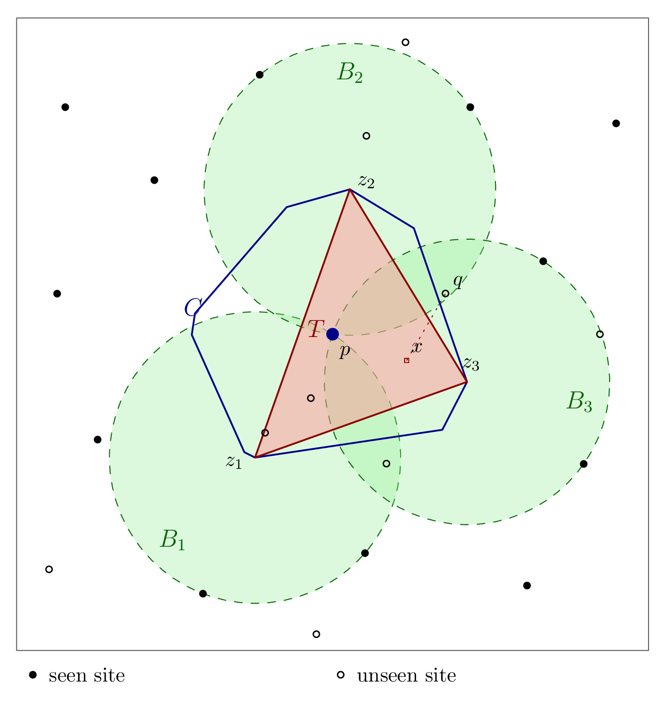
Figure 5: The triangle argument of [Lemma 4.2](#x1-420072): the disks $`B_j=B(z_j,\|z_j-p\|)`$ at the vertices of $`T\subseteq C`$ contain no seen site, and every unseen site that ends up owning a point $`x\in T`$, such as $`q`$, lies in one of them.
**Lemma 4.2 (Few owners of a triangle).** *In the* [*planar random-arrival setting*](#x1-150042)*, let* $`m=\lfloor n/2\rfloor`$ *and assume* $`n`$ *is sufficiently large. With probability at least* $`1-n^{-3}`$*, the following holds simultaneously for every* $`i\geq m`$ *and* $`p\in P_i`$*. The lifted current cell* $`C`$ *of* $`p`$ *contains a triangle* $`T`$ *with* $`\mathrm{area}\left(T\right)\geq \mathrm{area}\left(C\right)/4`$*, whose projection intersects at most* $`\kappa _0=c_0\log n`$ *final Voronoi cells in positive area, for an absolute constant* $`c_0`$*. The sites of these cells belong to* $`\{p\}\cup (P\setminus P_i)`$*.*
*Proof:* *Plan.* The logarithm comes from the random half: with high probability, no disk that is empty of the random prefix $`P_m`$ contains many sites of $`P`$, because there are only polynomially many disk-induced subsets. The final owners of a large triangle in the current cell, other than $`p`$ itself, all lie in three such empty disks, one around each vertex.
*Empty disks contain few sites.* With probability at least $`1-n^{-3}`$, every open torus disk empty of $`P_m`$ contains at most $`\kappa =c_1\log n`$ sites of $`P`$, for a sufficiently large constant $`c_1`$. Here it suffices to consider disks of radius at most $`\sqrt 2/2`$. To see this, take the nine translates of $`P`$ by vectors in $`\{-1,0,1\}^2`$. A torus disk is represented by an ordinary disk centered in $`[0,1]^2`$, and membership of a site means that at least one of its copies belongs to this disk. Ordinary disks induce $`O(n^3)`$ subsets on these $`9n`$ points: a disk with center $`(u,v)`$ and radius $`r`$ contains $`(x,y)`$ exactly when $`x^2+y^2-2ux-2vy+(u^2+v^2-r^2)<0`$, which is linear in the three parameters $`u`$, $`v`$, and $`u^2+v^2-r^2`$. Thus there are only $`O(n^3)`$ possible subsets of $`P`$ to consider. A fixed $`k`$-point subset avoids the uniform sample $`P_m`$ with probability at most $`(1-m/n)^k\leq (2/3)^k`$, for $`n\geq 3`$. A union bound proves the claim. In particular, it holds for every disk chosen later from the observed data.
*A large triangle.* Every convex polygon $`C`$ contains a triangle of at least a quarter of its area. Indeed, take a diameter $`z_1z_2`$, of length $`\ell`$, and a point $`z_3\in C`$ at the greatest distance $`\eta`$ from the line through $`z_1,z_2`$. A rectangle aligned with $`z_1z_2`$ and enclosing $`C`$ has width $`\ell`$ and height at most $`2\eta`$, while the triangle $`z_1z_2z_3`$ has area $`\ell \eta /2`$; so $`\mathrm{area}\left(C\right)\le 2\ell \eta =4\mathrm{area}\left(z_1z_2z_3\right)`$.
*Owners of the triangle.* Let $`T\subseteq C`$ be such a triangle, with vertices $`z_1,z_2,z_3`$. [Figure 5](#the-triangle-argument-of-lemmarandomorderownerslemmaref-lemmarandomorderowners-the-disks-bjbzjzjp-at-the-vertices-of-t-c-contain-no-seen-site-and-every-unseen-site-that-ends-up-owning-a-point-x-t-such-as-q-lies-in-one-of-them) shows the key containment: an unseen owner beating $`p`$ inside $`T`$ must lie in one of the disks centred at the vertices. The three open disks
```math
B_j=B\bigl (z_j,\|z_j-p\|\bigr ),\qquad j=1,2,3,
```
interpreted on the torus, are empty of $`P_i`$, because $`z_j`$ lies in the current cell of $`p`$ and so no site of $`P_i`$ is closer to $`z_j`$ than $`p`$; each therefore contains at most $`\kappa`$ final sites. If a final site $`q\ne p`$ owns a point $`x\in T`$ away from cell boundaries, let $`\widetilde q`$ be the periodic copy of $`q`$ closest to $`x`$. The function
```math
\|y-\widetilde q\|^2-\|y-p\|^2
```
is affine in $`y`$. It is negative at $`x`$, and therefore negative at some vertex $`z_j`$. Thus the site $`q`$ belongs to $`B_j`$. All final owners of $`T`$ consequently lie in $`\{p\}\cup \bigl (P\cap (B_1\cup B_2\cup B_3)\bigr )`$. There are at most $`1+3\kappa \leq \kappa _0`$ of them, and every owner other than $`p`$ is still unseen.
**The strategy.** Ignore the first $`m`$ sites and wait for the first trigger. Let $`p`$ be the triggering site. If no sites remain, select $`p`$. Otherwise, construct a triangle $`T`$ as in [Lemma 4.2](#x1-420072) in its current cell. Pick a point $`x`$ uniformly in $`T`$, and toss a fair coin. On heads, select $`p`$ immediately. On tails, run the usual secretary strategy on the remaining sites, with the fixed score $`-d_D(x,q)`$ for a site $`q`$. Concretely, ignore the first half of this remaining sequence and select the first later site closer to $`x`$ than every site in that half. This selects the nearest remaining site with probability at least $`1/4`$; if there is only one remaining site, the tails branch selects it. Whenever a rule would otherwise make no selection, select the last site. Coordinates of $`x`$ are understood modulo the torus.
**Theorem 4.3 (Logarithmic approximation).** *In the* [*planar random-arrival setting*](#x1-150042)*, there are a one-choice strategy and absolute constants* $`c_1,c_2>0`$ *such that, for every sufficiently large* $`n`$ *and every* $`n`$*-site input* $`P`$*,*
```math
{\mathbb{P}}\left[ Y\geq c_1M/\log n \right]\geq c_2.
```
*Thus the expected competitive ratio is* $`O(\log n)`$*. The strategy uses no information about* $`P`$ *beyond the arriving coordinates.*
*Proof:* Fix a final optimal site $`p^*`$. By [Lemma 4.1](#x1-420021), $`{\mathbb{P}}\left[ \tau =i\mid P_i \right]`$ does not depend on $`P_i`$, so conditioning on $`\tau =i`$ leaves $`P_i`$ a uniform $`i`$-point subset of $`P`$. Consequently,
```math
\begin{align*} {\mathbb{P}}\left[ \tau \leq n,\ p^*\in P_\tau \right] &=\sum _{i=m+1}^n{\mathbb{P}}\left[ \tau =i \right]\frac in \geq \frac mn{\mathbb{P}}\left[ \tau \leq n \right] =\frac mn\left (1-\frac mn\right ) =\Omega (1). \end{align*}
```
On this event, the triggering cell has area at least $`M`$: the current cell of $`p^*`$ contains its final cell, and the triggering cell is a largest current cell. Intersecting with the event of [Lemma 4.2](#x1-420072) loses at most $`n^{-3}`$ in probability.
Condition on a triggering prefix for which both events hold. Its triangle $`T`$ has area at least $`M/4`$ and at most $`\kappa _0`$ final owners. The final cells of area less than $`\mathrm{area}\left(T\right)/(2\kappa _0)`$ cover at most half of $`T`$. Therefore, with probability at least $`1/2`$, the final owner $`q`$ of the random point $`x`$ satisfies
```math
v(q)\geq \frac {\mathrm{area}\left(T\right)}{2\kappa _0}\geq \frac {M}{8\kappa _0}.
```
This owner is either $`p`$ or an unseen site. In the first case, the coin selects it with probability $`1/2`$. In the second, it is the closest unseen site to $`x`$. The unseen sites still arrive in uniformly random order, so the coin and the secretary strategy select it with probability at least $`(1/2)(1/4)=1/8`$. If there are no unseen sites, the owner is $`p`$ and is selected. The conditional probability of obtaining the displayed payoff is thus at least $`1/16`$. Since the required triggering prefixes occur with constant probability and $`\kappa _0=O(\log n)`$, the result follows.
### 4.2 An almost matching lower bound
The lower bound deletes a block of $`h`$ consecutive sites from a regular grid on the circle. The two sites bordering the gap own cells about $`h/2`$ times longer than every other cell, and until a short suffix remains, many unseen blocks are still plausible deletions. So early selections must guess the true block among many candidates, and late selections rarely see either valuable site. (With $`h=1`$, the same construction gives the exact-selection bound of [Lemma 4.11](#x1-5300111) below.)
**Theorem 4.4 (Lower bound for random order).** *In the* [*random-arrival model*](#x1-150042)*, on the circle or in the plane, for every sufficiently large* $`n`$*, every integer* $`1\leq b\leq \sqrt n`$*, and every possibly randomized* $`b`$*-choice strategy, there is a fixed* $`n`$*-site input* $`P\subset D`$ *with*
```math
\frac {{\mathbb{E}}\left[ Y \right]}M=O\left (\frac {\log \log n}{\log n}\right ).
```
*The implicit constant is absolute. Consequently the worst-case expected competitive ratio is* $`\Omega (\log n/\log \log n)`$*, even with this selection budget.*
*Proof:* Put
```math
h=\left \lfloor \frac {\log n}{4\log \log n}\right \rfloor , \qquad N=n+h, \qquad f=\left \lfloor \frac {n}{\log n}\right \rfloor .
```
Start with $`N`$ equally spaced positions on the unit circle and delete a uniformly random block of $`h`$ consecutive positions. Present the remaining $`n`$ sites in random order. We may tell the player the entire grid and the value of $`h`$. The two sites bordering the deleted block have cell length $`M=(h+2)/(2N)`$; all other cells have length $`1/N`$. Hence,
```math
\frac {{\mathbb{E}}\left[ Y \right]}{M} \leq \frac {2}{h+2}+{\mathbb{P}}\left[ \text {select a bordering site} \right].
\tag {7}
```
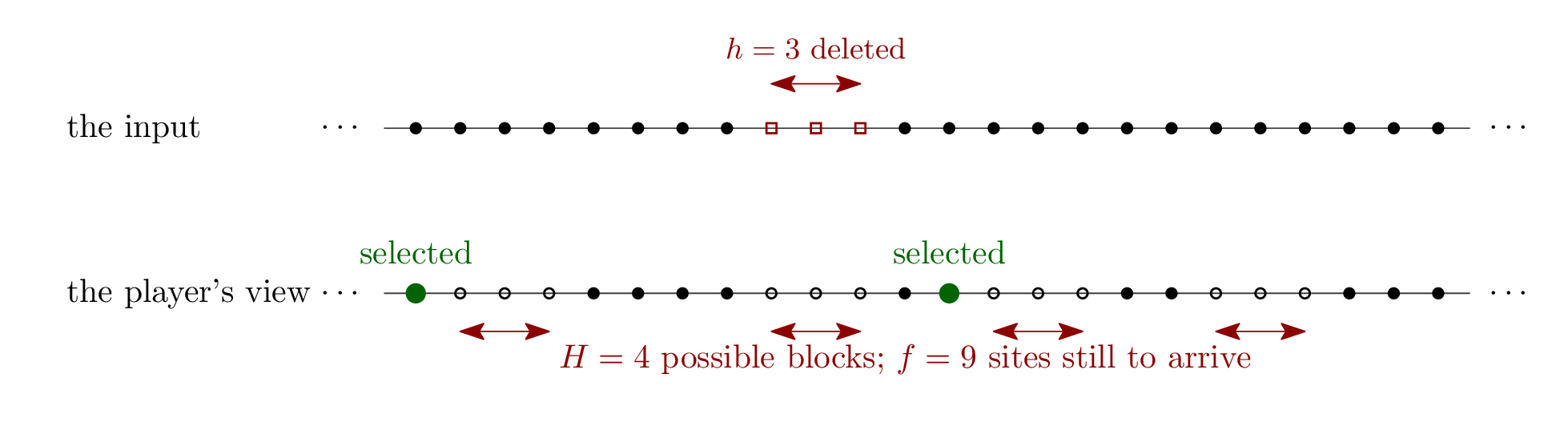
Figure 6: The deleted-block instance at the cutoff, with $`N=24`$, $`h=3`$, and $`f=9`$ sites still to arrive: the input (top) and what the player has seen (bottom), where the $`H=4`$ possible blocks look alike.
Examine the prefix when $`f`$ arrivals remain. Call a block of $`h`$ consecutive grid positions *possible* if none of its positions has appeared, and let $`H`$ be the number of possible blocks ([Figure 6](#the-deletedblock-instance-at-the-cutoff-with-n24-h3-and-f9-sites-still-to-arrive-the-input-top-and-what-the-player-has-seen-bottom-where-the-h4-possible-blocks-look-alike)). All possible blocks are equally likely to be the true deleted block: each gives the observed ordered prefix the same likelihood. The sites selected so far border at most $`2b`$ possible blocks, so on $`H\geq n^{2/3}`$ their conditional probability of including a bordering site is at most $`2b/n^{2/3}`$; the event $`H
```math
{\mathbb{P}}\left[ \text {select a bordering site} \right] \leq \frac {2b}{n^{2/3}} +{\mathbb{P}}\left[ H
### 4.3 Sublinear selection budgets
The obstruction persists for every sublinear budget. A regular polygon of nearby sites shares a grid cell; deleting all but one vertex leaves a valuable survivor whose identity is difficult to infer online. Write $`M_2`$ for the second-largest final cell and $`\Gamma =M/M_2`$.
There are two requirements on the construction. Geometrically, the exceptional survivor must be substantially better than every ordinary site, so that failing to select it entails a large loss. Informationally, many ordinary clusters must still look exceptional when a decision is made. The parameter $`k`$ controls both effects: larger clusters increase the possible area advantage but also create more arrivals that can reveal that a cluster is ordinary. [Theorem 4.5](#x1-450015) quantifies this balance, and [Corollary 4.6](#x1-470016) chooses $`k`$ as a function of the available budget. The lower bound gives the player all potential site positions, so the uncertainty lies in the missing sites rather than in the geometry of the candidate family.
**Theorem 4.5 (Budget tradeoff).** *In the* [*planar random-arrival setting*](#x1-150042)*, for every sufficiently large* $`n`$*, integers* $`3\leq k\leq \log n`$ *and* $`1\leq b\leq n`$*, and every strategy selecting at most* $`b`$ *sites, there is an* $`n`$*-site instance on* $`\mathbb T^2`$ *with a unique optimum, gap* $`k/3\leq \Gamma \leq 2k`$*, and*
```math
{\mathbb{P}}\left[ \text {select the optimum} \right] \leq \min \{1,25(bk/n)^{1/k}\},\qquad \frac {{\mathbb{E}}\left[ Y \right]}M\leq \frac 3k+25(bk/n)^{1/k}.
\tag {9}
```
*The strategy may know the entire family of possible instances.*
*Proof:* Put $`m=\lfloor \sqrt {n/k}\rfloor`$, $`w=1/m`$, $`A=w^2`$, and $`\rho =w/(1000k)`$. At each center of an $`m\times m`$ square torus grid place a regular $`k`$-gon of radius $`\rho`$, with a common orientation and one designated vertex. Reserve one cluster for padding. Choose one of the other $`m^2-1`$ clusters uniformly and delete its $`k-1`$ nondesignated vertices. Finally place $`n-km^2+k-1`$ distinct additional sites within distance $`\rho /100`$ of the padding center. The resulting instance has exactly $`n`$ sites. All potential positions and designated vertices are disclosed. In [Figure 7](#the-cluster-construction-with-k5-and-exaggerated-ordinary-clusters-share-their-grid-square-the-exceptional-cluster-keeps-only-its-designated-vertex-whose-cell-shaded-is-almost-the-whole-square-its-other-vertices-hollow-being-absent-padding-not-shown), compare the survivor’s nearly full grid square with the narrow cells around each intact polygon. Online, an ordinary cluster of which only the designated vertex has arrived looks exactly like the exceptional one.
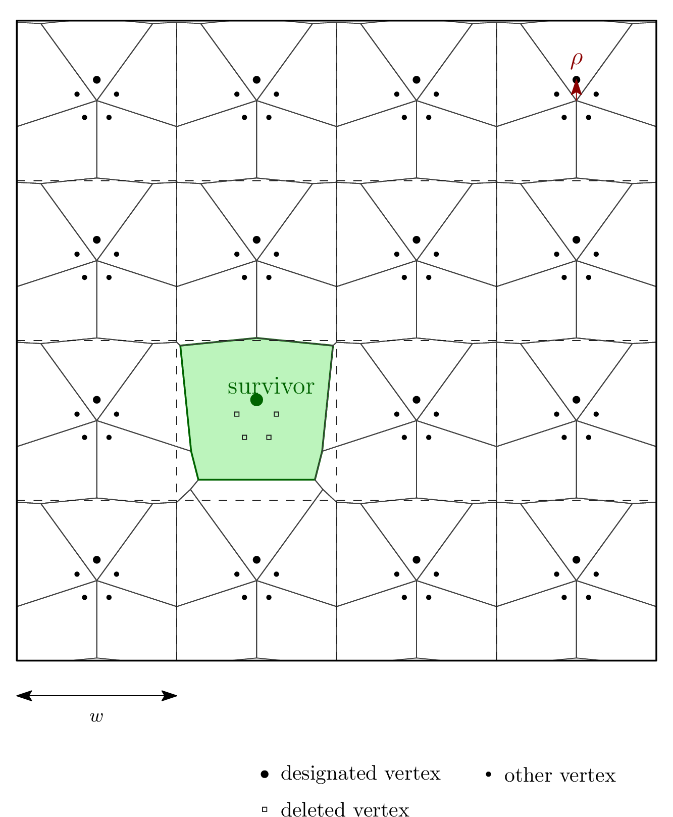
Figure 7: The cluster construction with $`k=5`$ and $`\rho`$ exaggerated. Ordinary clusters share their grid square; the exceptional cluster keeps only its designated vertex, whose cell (shaded) is almost the whole square, its other vertices (hollow) being absent. Padding not shown.
**Geometry.** We show three things: every ordinary cell is small, the survivor owns almost a full grid square, and the padding changes neither fact. All statements use periodic lifts; for all sufficiently large $`n`$ the disks involved have radius less than $`1/4`$, so torus and Euclidean distances agree inside them.
*Ordinary cells.* First consider the full configuration, with every cluster intact and no padding. By translation symmetry, each cluster owns total area $`A`$. Within a cluster, the competitors of a vertex lie on a regular $`k`$-gon around the center $`z_0`$, so its cell lies in an angular sector of angle $`2\pi /k`$ about $`z_0`$. Every point has a grid center within distance $`w/\sqrt 2`$, hence a site within distance $`w/\sqrt 2+\rho`$; a point owned by a vertex of the cluster at $`z_0`$ is therefore within distance $`w/\sqrt 2+2\rho`$ of $`z_0`$. So every cell has area at most
```math
\frac {\pi }{k}(w/\sqrt 2+2\rho )^2.
```
*The survivor.* Now delete the nondesignated vertices of the cluster at $`z_0`$. We claim that the survivor owns the square $`z_0+[-w/2+4\rho ,w/2-4\rho ]^2`$. Take $`z_0`$ as origin, let $`x`$ be a point of this square, and let $`z=w(i,j)\ne 0`$ be any other lifted grid center, with $`\ell =|i|+|j|\geq 1`$. Then
```math
\|x-z\|^2-\|x\|^2\geq 8w\rho \ell , \qquad \|x-z\|+\|x\|\leq w(\ell +\sqrt 2)\leq 3w\ell ,
```
so $`\|x-z\|-\|x\|\geq 8\rho /3>2\rho`$. Every site lies within $`\rho`$ of its grid center, so $`x`$ is strictly closer to the survivor than to every site of every other cluster, proving the claim. Deleting sites only transfers area: a point whose nearest site survives keeps its owner. Hence the survivor’s cell lies in the territory of area $`A`$ that its cluster owned before the deletion, and the cells of all other sites grow only by parts of that territory not owned by the survivor. Writing $`M_0`$ for the survivor’s area at this stage,
```math
A-16w\rho \leq (w-8\rho )^2\leq M_0\leq A,
```
and the total growth of all other cells is at most $`A-M_0\leq 16w\rho`$. Each ordinary cell therefore has area at most
```math
\frac {\pi }{k}(w/\sqrt 2+2\rho )^2+16w\rho <\frac {2A}{k}.
```
*Padding.* Adding the padding sites only shrinks existing cells, and the survivor still owns its inset square, since the comparison above covers every site within $`\rho`$ of the padding center. Each padding cell lies within distance $`2\rho`$ of the padding center. To see this, translate the padding center to the origin, write $`p`$ for a padding site, and take a lift $`x`$ with $`\|x\|\geq 2\rho`$. Some vertex $`y`$ of the intact ring at the padding center has projection at least $`\rho \cos (\pi /k)\geq \rho /2`$ in the direction of $`x`$, whereas $`\|p\|\leq \rho /100`$. Hence
```math
\|x-y\|^2-\|x-p\|^2 \leq \rho ^2-2\|x\|(\rho /2-\rho /100)<0,
```
so $`x`$ is not owned by $`p`$. A padding cell thus has area at most $`4\pi \rho ^2<2A/k`$.
*The gap.* The exceptional survivor is the unique optimum, with final area $`.99A\leq M\leq A`$, while every other cell has area less than $`2A/k`$; hence $`\Gamma \geq k/3`$. For the other direction, for $`m\geq 3`$ we have $`n-1 **Information.** It suffices to consider $`bk
**Corollary 4.6 (Linear budgets).** *In the* [*planar random-arrival setting*](#x1-150042)*, let* $`b=b(n)`$ *and* $`r=n/b\to \infty`$*. Every* $`b`$*-choice strategy has a fixed planar torus instance with a unique optimum and*
```math
\frac {{\mathbb{E}}\left[ Y \right]}M=O\left (\frac {\log \log r}{\log r}\right ).
```
*Consequently, constant expected competitiveness for arbitrary fixed planar sites requires and is achievable with* $`\Theta (n)`$ *choices.*
*Proof:* For the lower bound, take the cluster size $`k`$ as large as the second term in [Theorem 4.5](#x1-450015) allows. For sufficiency, accept the first $`b`$ arrivals. Take $`k=\lfloor \log r/(4\log \log r)\rfloor`$, which lies between $`3`$ and $`\log n`$ for sufficiently large $`r`$. Since $`\log r-\log k\geq (3/4)\log r`$ eventually,
```math
(k/r)^{1/k} \leq \exp (-3\log \log r)=(\log r)^{-3}.
```
Apply [Theorem 4.5](#x1-450015). If a budget is not $`\Omega (n)`$, it has a subsequence with $`n/b\to \infty`$, ruling out a uniform constant guarantee. Conversely, selecting the first $`b`$ arrivals includes any fixed optimum with probability $`b/n`$, and so gives $`{\mathbb{E}}\left[ Y \right]\geq (b/n)M`$.
**Large gaps are easy.** The cluster instances have gap $`\Gamma \le 2k\le 2\log n`$. The next theorem shows that this is the right scale: once the optimum is larger than every other cell by a factor of order $`\log n`$, a logarithmic budget captures it with constant probability, and a larger gap gives success probability tending to one. The strategy is the greedy one, and it needs to know neither $`\Gamma`$ nor the input.
**Theorem 4.7 (Large gaps).** *In the* [*planar random-arrival setting*](#x1-150042)*, let the input have a unique optimum* $`p^*`$*, let* $`M_2`$ *be the second-largest final cell, and write* $`\Gamma =M/M_2`$*. Select every arriving site whose cell is largest in the current diagram, breaking ties by a fixed order, until* $`b=\lceil c_1\log n\rceil`$ *sites have been selected. For suitable absolute constants* $`c_1,c_2`$ *and all sufficiently large* $`n`$*,*
```math
{\mathbb{P}}\left[ p^*\text { is selected} \right] \geq \exp \left (-\frac {c_2\log n}{\Gamma }\right )-\frac 2n.
```
*In particular, a gap of order* $`\log n`$ *gives constant success probability, and if* $`\Gamma /\log n\to \infty`$ *then* $`p^*`$ *is selected with probability* $`1-O(\log n/\Gamma )`$*; here* $`\Gamma \le n-1`$*, since* $`M\le 1/2`$ *and* $`M_2\ge (1-M)/(n-1)`$*.*
*Proof:* *Plan.* The stopping identity bounds the number of triggering arrivals, so a logarithmic budget is unlikely to run out. In a late suffix, every disk empty of the prefix contains few final sites, and the triangle argument then bounds every competing current cell below $`M`$; so if $`p^*`$ arrives in that suffix, it triggers and, unless the budget has run out, is selected.
By [Lemma 4.1](#x1-420021), the number of triggering arrivals, those whose current cell is largest at their arrival, is a sum of independent indicators with mean $`\sum _{i=1}^n1/i\leq 1+\log n`$. A Chernoff bound makes the probability that this number exceeds $`b`$ at most $`n^{-3}`$, for a sufficiently large $`c_1`$. If $`p^*`$ triggers at its arrival but the budget is already exhausted, then more than $`b`$ sites triggered; so, except with probability $`n^{-3}`$, the budget never prevents the selection of $`p^*`$.
Put $`\phi =\exp (-c_2\log n/\Gamma )`$ and $`f=\lfloor n\phi \rfloor`$. If $`f=0`$ then $`\phi <1/n`$ and the asserted bound is negative, so assume $`f\geq 1`$, which forces $`\Gamma \geq c_2`$. Consider the prefix of the first $`n-f`$ sites. Rerun the disk-range argument from the proof of [Lemma 4.2](#x1-420072) with this prefix in place of $`P_m`$: a fixed $`\kappa`$-point subset of $`P`$ avoids it with probability at most $`(f/n)^\kappa \leq \phi ^\kappa`$, and there are $`O(n^3)`$ disk-induced subsets. Hence, except with probability at most $`n^{-3}`$, every open torus disk that is empty of the prefix contains fewer than
```math
\kappa =\left \lceil \frac {c_3\log n}{\log (1/\phi )}\right \rceil \leq \frac {c_3\Gamma }{c_2}+1
```
final sites, for a sufficiently large absolute constant $`c_3`$.
Suppose that $`p^*`$ arrives after the prefix, and look at the current diagram at that moment. Let $`C`$ be the lifted current cell of any other site $`p`$. By the triangle argument in the proof of [Lemma 4.2](#x1-420072), $`C`$ contains a triangle $`T`$ of area at least $`\mathrm{area}\left(C\right)/4`$ whose final owners lie in $`\{p\}`$ and in three open disks that are empty of the current prefix, hence of the first $`n-f`$ sites; so $`T`$ has fewer than $`3\kappa`$ final owners. None of them is $`p^*`$, whose final cell lies inside its own current cell, disjoint from the interior of $`C`$. Every final owner of $`T`$ thus has final area at most $`M_2`$, and
```math
\mathrm{area}\left(C\right)\leq 4\mathrm{area}\left(T\right)<12\kappa M_2 \leq \left (\frac {12c_3\Gamma }{c_2}+12\right )M_2<\Gamma M_2=M,
```
once $`c_2\geq 48c_3`$ and $`c_2\geq 48`$, using $`\Gamma \geq c_2`$. The current cell of $`p^*`$ contains its final cell and so has area at least $`M`$. Therefore $`p^*`$ is the unique triggering site at its arrival and is selected unless the budget is exhausted. It arrives after the prefix with probability $`f/n\geq \phi -1/n`$. Subtracting the two failure probabilities of $`n^{-3}`$ each proves the theorem.
### 4.4 The missing-vertex game on a circle
The following game concerns graph adjacency, not Voronoi-cell selection, but it seems to capture the Voronoi game behavior at some simple settings where one must name the largest cell.
Problem 4.8 (One missing vertex). The player knows a finite simple undirected graph $`G=(V,E)`$ with $`N=|V|\geq 2`$ and $`E\ne \emptyset`$. A random permutation of the vertices is chosen with the last one being designated as $`J`$. The permutation is revealed one by one. On an arrival $`v_t`$, the $`t`$th vertext in the permutation, the player may either continue or make its single irrevocable guess, naming one still-unseen vertex adjacent to $`v_t`$ as being $`J`$. A correct guess wins, while an incorrect name or no guess loses. The player knows $`G`$ in advance, and the revealed identities. Randomized strategies are allowed.
**Notations.** Let $`p_G`$ be the maximum probability of a win for the player over all randomized strategies. For the random permutation underlying the game, let $`U_t=V\setminus \{v_1,\ldots ,v_t\}`$ be the $`t`$-suffix of the permutation. Let $`\sigma =\min \left\{ t \;\middle\vert\; E(G[U_t])=\emptyset \right\}`$ the first time no two missing vertices are adjacent. Thus, $`K=|U_\sigma |`$ is the number of missing vertices at this point in time.
Consider the [missing-vertex game](#x1-490018) played on the cycle of length $`n`$: $`G=C_N`$, $`N\geq 3`$. The player must name the hidden vertex upon the arrival of one of its graph neighbors. The question is how much the gradually accumulating evidence helps.
**The strategy.** Wait until the unseen positions contain no consecutive pair, and then guess an unseen neighbor of the position just revealed (i.e., think about the situation where the graph is a grid).
**Lemma 4.9.** *In the* [*missing-vertex game*](#x1-490018) *on the cycle graph* $`G=C_n`$*, consider the strategy that waits until time* $`\sigma`$*, when the last edge in the unseen induced graph disappears, and guesses any unseen neighbor of the vertex that arrived at that time. Its success probability is* $`p_G = {\mathbb{E}}\left[ 1/K \right],`$ *where* $`K`$ *is the number of holes remaining at this point in time.*
*Proof:* Use backward analysis—fix the $`n-K`$ first elements in the permutation. Think about the suffix of the permutation as not being determined yet. The player chooses one of the holes at this point in time. But $`J`$ has a uniform distribution over the holes, so the probability the player won is $`1/K`$. Now average this success probability over all possible permutations.
As for the optimality—a strategy that stops earlier, say where there are $`\ell > K`$ holes, has success probability at most $`1/\ell < 1/K`$. Stopping later is not an option as this is the last iteration in which the player can make a choice.
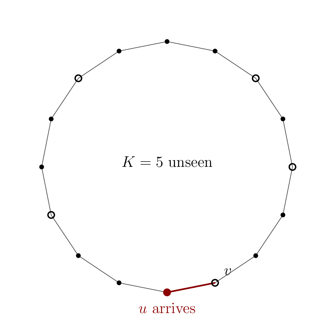
Figure 8: The missing-vertex game on $`C_{16}`$ at the moment the optimal rule guesses: the only unseen (hollow) adjacent pair was $`\{u,v\}`$, and $`u`$ has arrived, so the player names $`v`$, which is correct with probability $`1/K=1/5`$.
XXX
**Why the square-root scale?** [Figure 8](#the-missingvertex-game-on-c16-at-the-moment-the-optimal-rule-guesses-the-only-unseen-hollow-adjacent-pair-was-uv-and-u-has-arrived-so-the-player-names-v-which-is-correct-with-probability-1k15) shows the moment at which the strategy stops. The probability that a specific edge on the cycle has the ultimate and penultimate vertices in the permutation is $`1/\binom {N}{2}`$. With $`k`$ positions still unseen, the probability this specific edge to be connected by two of unseen indices is thus $`\binom {k}{2}/\binom {N}{2}`$. Since there are $`N`$ edges, we get that the expected number of edges still alive is $`N\binom {k}{2} / \binom {N}{2} = k(k-1)/(N-1)`$. This quantity is roughly $`1`$ for $`k=\sqrt {N}`$, and we expect $`K`$ to be roughly $`\sqrt {N}`$. Informally, the probability of success is the inverse of $`K`$, which is (roughly) $`1/\sqrt {N}`$.
**Theorem 4.10 (The cycle).** *In the* [*missing-vertex game*](#x1-490018) *with* $`G=C_N`$ *and* $`N\to \infty`$*, the optimal success probability is*
```math
p_{C_N}=\frac {\sqrt \pi +o(1)}{\sqrt N}.
```
*For every* $`N\geq 3`$*, the number* $`K`$ *of vertices left unseen when the last unseen edge disappears satisfies*
```math
{\mathbb{P}}\left[ K\geq k \right] =\frac {N}{N-k}\frac {\binom {N-k}{k}}{\binom Nk}, \qquad 1\leq k\leq \lfloor N/2\rfloor ,
```
*and this probability is zero for larger* $`k`$*.*
*Proof:* Append $`J`$ to the arrival sequence. The resulting order is a uniform permutation of all $`N`$ vertices. Read it backwards. Its first $`K`$ vertices contain no adjacent pair, and the next vertex creates the first such pair. Consequently, $`{\mathbb{P}}\left[ K\geq k \right]`$ is the probability that a uniform $`k`$-subset of the cycle is independent.
The number of independent $`k`$-subsets is $`N\binom {N-k-1}{k-1}/k`$: distinguish one chosen vertex; the $`k`$ gaps then contain positive numbers of unchosen vertices summing to $`N-k`$, which gives $`\binom {N-k-1}{k-1}`$ ordered gap lists and $`N`$ choices of the distinguished vertex, and each set is counted $`k`$ times. This is $`\frac {N}{N-k}\binom {N-k}{k}`$, proving the exact formula. Writing the tail as
```math
{\mathbb{P}}\left[ K\geq k \right] =\prod _{j=1}^{k-1}\left (1-\frac {k}{N-j}\right )
```
and taking logarithms gives
```math
{\mathbb{P}}\left[ K\geq k \right] =\exp \left (-\frac {k(k-1)}{N} +O\left (\frac {k^3}{N^2}\right )\right )
```
for $`k=O(\sqrt N)`$. Hence $`K/\sqrt N`$ converges in distribution to a nonnegative random variable $`\zeta`$ with $`{\mathbb{P}}\left[ \zeta >x \right]=e^{-x^2}`$ for $`x\geq 0`$.
To pass to inverse expectations, a union bound over the cycle edges gives $`{\mathbb{P}}\left[ K\leq k \right]\leq k(k+1)/(N-1)`$. Fix $`\delta \in (0,1)`$ and $`\xi >1`$. Summation by parts therefore yields, for $`a=\lfloor \delta \sqrt N\rfloor`$,
```math
{\mathbb{E}}\left[ \frac {\sqrt N}{K}\,\mathbf 1_{K\leq a} \right] =O(\delta +N^{-1/2}).
```
On $`K>\xi \sqrt N`$, the same random variable is at most $`1/\xi`$. Truncation now justifies convergence of expectations, and
```math
\sqrt N\,p_{C_N}\to {\mathbb{E}}\left[ 1/\zeta \right]=\int _0^\infty 2e^{-x^2}\,dx=\sqrt \pi .
```
#### 4.4.1 A Voronoi consequence
On a regular circle grid with one position deleted, the two neighbors of the deleted position have the largest cells. A successful guess in the cycle game therefore yields a successful selection, by accepting the arriving neighbor; conversely, an optimal selected site has the missing position among its at most two unseen neighbors, so naming one of them at random is correct with probability at least one half.
**Lemma 4.11 (Exact selection on a deleted grid).** *Consider the* [*circle random-arrival setting*](#x1-150042) *with one choice and the following distribution over the unknown input. Let* $`\mathcal G`$ *consist of* $`n+1`$ *equally spaced positions on the unit circle. Delete a uniformly random position of* $`\mathcal G`$*, and present the remaining* $`n`$ *sites in random order. Even if the player knows* $`\mathcal G`$*, the optimal probability of selecting a largest final Voronoi cell is* $`\Theta (n^{-1/2})`$*, averaging over the deletion, arrival order, and strategy randomness.*
*Proof:* The two neighbors of the missing position are precisely the optimal sites. A strategy for the missing-vertex game yields a selection strategy with at least the same success probability: select the arriving site when the game strategy makes its guess. Conversely, simulate any selection strategy and, on its selected arrival, name a uniformly random unseen grid neighbor, if one exists. Whenever the selected site is optimal, this guess is correct with probability at least $`1/2`$. Thus the two optimal success probabilities differ by at most a factor of two. Apply [Theorem 4.10](#x1-5200110) with $`N=n+1`$.
Both optimal cells have length $`3/(2(n+1))`$, and every other cell has length $`1/(n+1)`$. Thus, for every $`1\leq \alpha <3/2`$, obtaining a payoff at least $`M/\alpha`$ requires selecting an optimal site and has probability $`O(n^{-1/2})`$. The expected payoff is at most $`(2/3+O(n^{-1/2}))M`$.
#### 4.4.2 Missing vertices on general graphs
The optimal rule in [Lemma 4.9](#x1-510019) applies to every known graph. Its exact value is governed by the number of independent sets of each size, rather than by the maximum size of an independent set.
**Proposition 4.12 (Independent-set formula).** *In the* [*missing-vertex game*](#x1-490018)*, let* $`i_k(G)`$ *be the number of independent* $`k`$*-subsets of the known graph* $`G`$*. With* $`N,K,p_G`$ *as defined there, for every integer* $`1\leq k\leq N`$*,*
```math
{\mathbb{P}}\left[ K\geq k \right]=\frac {i_k(G)}{\binom Nk}, \qquad p_G=\sum _{k=1}^{N-1}\frac 1k \left (\frac {i_k(G)}{\binom Nk} -\frac {i_{k+1}(G)}{\binom N{k+1}}\right ).
```
*Proof:* Append the missing vertex to the arrivals and read the resulting uniform permutation backwards, as in [Theorem 4.10](#x1-5200110). The first $`k`$ vertices are independent exactly when $`K\geq k`$. The second identity is $`{\mathbb{E}}\left[ 1/K \right]`$ written using these tail probabilities.
The proof of the next theorem has two parts. First, at the scale $`s=\sqrt {N/d}`$, the number of edges inside a uniformly random $`k`$-set is asymptotically Poisson, which gives the limit law of $`K/s`$. Second, a union bound over edges controls the probability that $`K/s`$ is small, where the scaled payoff $`s/K`$ becomes large; this justifies the convergence of $`{\mathbb{E}}\left[ s/K \right]`$.
**Theorem 4.13 (Regular graphs).** *In the* [*missing-vertex game*](#x1-490018)*, for every sequence of known* $`d`$*-regular graphs* $`G`$ *on* $`N\to \infty`$ *vertices with* $`1\leq d=o(N)`$*, the optimal one-guess success probability is*
```math
p_G=\left (\sqrt {\frac \pi 2}+o(1)\right )\sqrt {\frac dN}.
```
*Proof:* Put $`s=\sqrt {N/d}`$, which tends to infinity. Let $`X_k`$ count the edges in a uniform $`k`$-subset of vertices. For $`k=\lfloor xs\rfloor`$ and fixed $`x>0`$,
```math
{\mathbb{E}}\left[ X_k \right]=\frac {Nd}{2}\frac {(k)_2}{(N)_2} \to \frac {x^2}{2}.
```
In fact, $`X_k`$ converges to a Poisson random variable with this mean. Here is a factorial-moment proof. For a fixed positive integer $`r`$, the ordered $`r`$-tuples of vertex-disjoint edges contribute $`(x^2/2)^r+o(1)`$ to $`{\mathbb{E}}\left[ (X_k)_r \right]`$: their number is $`(1+o(1))(Nd/2)^r`$, and each tuple is included with probability $`(k)_{2r}/(N)_{2r}`$.
Group the remaining ordered $`r`$-tuples of distinct edges by the pattern of shared endpoints among them. For one such pattern, let $`w`$ be the number of vertices and $`\ell`$ the number of connected components of the union of its edges; there are finitely many patterns for fixed $`r`$. Choosing a root in each component and embedding spanning trees bounds the number of tuples with this pattern by $`O_r(N^\ell d^{w-\ell })`$. Its contribution to the factorial moment is at most
```math
O_r\left (N^\ell d^{w-\ell }(k/N)^w\right ) =O_{r,x}\left ((d/N)^{w/2-\ell }\right )=o(1),
```
since every component has at least two vertices and at least one has three or more. This proves the Poisson limit by factorial moments. Therefore
```math
{\mathbb{P}}\left[ K\geq \lfloor xs\rfloor \right] ={\mathbb{P}}\left[ X_{\lfloor xs\rfloor }=0 \right] \to e^{-x^2/2}.
```
A union bound over edges gives $`{\mathbb{P}}\left[ K\leq k \right]\leq d\,k(k+1)/(2(N-1))`$. To justify passing from the distributional limit to the inverse expectation, fix $`\delta \in (0,1)`$ and $`\xi >1`$, put $`\Phi (k)={\mathbb{P}}\left[ K\leq k \right]`$ and $`a=\lfloor \delta s\rfloor`$. For $`a\geq 1`$, summation by parts gives
```math
{\mathbb{E}}\left[ \frac {s}{K}\mathbf 1_{K\leq a} \right] =s\left (\frac {\Phi (a)}a+ \sum _{k=1}^{a-1}\frac {\Phi (k)}{k(k+1)}\right ) =O(a/s)=O(\delta ),
```
using $`\Phi (k)\leq ck(k+1)/s^2`$ with an absolute constant $`c`$. For $`a=0`$ the expectation is zero. The contribution from $`K>\xi s`$ is at most $`1/\xi`$. On the remaining range $`\delta
**Corollary 4.14 (Examples).** *In the* [*missing-vertex game*](#x1-490018)*, on the square torus grid* $`C_m\square C_m`$*, the Cartesian product of two cycles, in which every vertex has degree* $`4`$ *and* $`N=m^2\to \infty`$*, the optimal success probability is* $`(\sqrt {2\pi }+o(1))/\sqrt N`$*. On the* $`d`$*-dimensional hypercube, with* $`N=2^d`$ *and degree* $`d`$*, it is* $`(\sqrt {\pi /2}+o(1))\sqrt {\log _2 N/N}`$*. Fixed-degree regular expanders have the same leading asymptotic as all other regular graphs of that degree.*
*Proof:* Apply [Theorem 4.13](#x1-5400513) with $`d=4`$, $`d=\log _2 N`$, and fixed $`d`$, respectively.
## 5 Concluding remarks
Several questions remain open.
1\.
For fixed sites in random order, one choice gives an $`O(\log n)`$ approximation, while the lower bound is $`\Omega (\log n/\log \log n)`$. Which is tight?
2\.
The best universal expected competitive factor for known laws on the circle lies between $`2`$ ([Theorem 3.6](#x1-280026)) and $`7000`$ ([Theorem 3.11](#x1-3600111)). The true constant is presumably small.
3\.
Does every known planar distribution admit a constant expected competitive ratio? The one-dimensional argument uses a length scale that controls the largest gap; in the plane, large empty regions need not correspond to attainable cell areas, and we do not know how to choose the regions to monitor.
4\.
In the plane, constant expected competitiveness for fixed sites in random order requires $`\Theta (n)`$ selections. We do not know the corresponding threshold on the circle, where every cell is determined by two gaps and the cluster construction does not apply.
5\.
The uniform results should extend to higher dimensions, with the leading constant of the largest Poisson–Voronoi cell replaced by its $`d`$-dimensional analogue, but we have not carried this out.
## A An elementary proof of the large-cell tail
We prove [Lemma 3.3](#x1-220013) without the roundness theorem. The argument uses only convexity and the Poisson empty-region probability. Let $`C`$ be the cell of the inserted origin in a unit-intensity planar Poisson process, so that $`\mathrm{area}\left(C\right)`$ is the area $`A`$ of [Lemma 3.3](#x1-220013). The key observation is that the interior of the doubled cell $`2C`$ contains no Poisson site. We first bound cells that extend far from the origin by a finite family of empty disks; for the remaining bounded cells, a grid supplies finitely many inner approximations whose doubles are empty.
**Observation A.1.** *For the cell* $`C`$ *of the inserted origin, the interior of* $`2C=\{2x:x\in C\}`$ *contains no Poisson site.*
*Proof:* If a site $`q`$ belonged to $`\operatorname {int}(2C)`$, then $`q/2`$ would be an interior point of $`C`$. But $`q/2`$ lies on the bisector of $`0`$ and $`q`$, and hence cannot be interior to the origin’s cell.
Consequently, a cell of area at least $`a`$ gives an empty region of area at least $`4a`$. To use the empty-region probability, we replace this random region by one of finitely many deterministic regions.
**Long cells.** Set $`R_0=4\sqrt a`$ and choose a fixed finite set $`U`$ of unit vectors such that every unit vector is within Euclidean distance $`1/4`$ of some member of $`U`$. If $`C`$ reaches distance $`R_0`$ from the origin, convexity gives $`R_0u\in C`$ for some unit vector $`u`$. The open disk $`B(R_0u,R_0)`$ contains no Poisson site. Choosing $`v\in U`$ with $`\|u-v\|\leq 1/4`$, it contains $`B(R_0v,3R_0/4)`$, which also excludes the inserted origin. Therefore
```math
{\mathbb{P}}\left[ C\not \subset B(0,R_0) \right] \le |U|e^{-9\pi R_0^2/16} =|U|e^{-9\pi a}.
\tag {10}
```
Null boundary events do not affect this estimate.
**Bounded cells.** Fix $`\delta \in (0,1)`$ and use a square grid of side $`s=c\delta \sqrt a`$, anchored at the origin; $`c>0`$ is a sufficiently small absolute constant. For a convex $`C\subset B(0,R_0)`$, let $`W`$ be the union of the closed grid squares contained in $`\operatorname {int}C`$. All points of $`C\setminus W`$ lie within distance $`\sqrt 2s`$ of $`\partial C`$.
Here is a direct bound on the lost area. A convex body in $`B(0,R_0)`$ has perimeter $`\ell \le 2\pi R_0`$: Cauchy’s perimeter formula integrates its projection widths, each at most $`2R_0`$. Mark boundary points at arclength gaps at most $`s`$. At most $`\ell /s+1`$ disks of radius $`3s`$ around these points cover the entire inner boundary strip of width $`\sqrt 2s`$. Thus
```math
\mathrm{area}\left(C\setminus W\right)\le 9\pi (\ell s+s^2)\le \delta a
```
by the choice of $`c`$. In particular, if $`\mathrm{area}\left(C\right)\ge a`$, then $`\mathrm{area}\left(W\right)\ge (1-\delta )a`$.
Only $`O((R_0/s+1)^2)=O(\delta ^{-2})`$ grid squares meet $`B(0,R_0)`$. Their subcollections give at most $`2^{O(\delta ^{-2})}`$ possible unions $`W`$. For every possible $`W`$ of area at least $`(1-\delta )a`$, the event $`W\subset \operatorname {int}C`$ forces the fixed region $`2W`$ to contain no Poisson site, by [Lemma A.1](#x1-560011); so $`{\mathbb{P}}\left[ W\subset \operatorname {int}C \right] \leq {\mathbb{P}}\left[ 2W\text { contains no Poisson site} \right] \leq e^{-4(1-\delta )a}`$, where the inserted origin, not being part of the Poisson process, does not affect the bound. Taking a union bound and using [Eq. (10)](#x1-57001r10), we obtain
```math
{\mathbb{P}}\left[ \mathrm{area}\left(C\right)\ge a \right] \le 2^{O(\delta ^{-2})}e^{-4(1-\delta )a} +|U|e^{-9\pi a}.
```
This proves the upper bound in [Lemma 3.3](#x1-220013); its lower bound is the empty disk $`B(0,2\sqrt {a/\pi })`$. In particular, $`\log {\mathbb{P}}\left[ \mathrm{area}\left(C\right)\ge a \right]/a\to -4`$.
## References
\[ACC+04\]
H.-K. Ahn, S.-W. Cheng, O. Cheong, M. Golin, and R. van Oostrum. [Competitive facility location: the Voronoi game](http://dx.doi.org/10.1016/j.tcs.2003.09.004). *Theo. Comp. Sci.*, 310: 457–467, 2004.
\[BF93\]
F. T. Bruss and T. S. Ferguson. [Minimizing the expected rank with full information](http://dx.doi.org/10.2307/3214770). *J. Appl. Probab.*, 30(3): 616–626, 1993.
\[BHMM16\]
M. Boppana, R. Hod, M. Mitzenmacher, and T. Morgan. [Voronoi choice games](http://dx.doi.org/10.4230/LIPICS.ICALP.2016.23). *Proc. 42nd Int. Colloq. Automata Lang. Prog.* (ICALP)*,* vol. 55. 23:1–23:13, 2016.
\[Bru05\]
F. T. Bruss. [What is known about Robbins’ problem?](http://dx.doi.org/10.1239/jap/1110381374) *J. Appl. Probab.*, 42(1): 108–120, 2005.
\[CD22\]
R. L. Church and Z. Drezner. [Review of obnoxious facilities location problems](http://dx.doi.org/10.1016/j.cor.2021.105468). *Comput. & Oper. Res.*, 138: 105468, 2022.
\[CFH+19\]
J. Correa, P. Foncea, R. Hoeksma, T. Oosterwijk, and T. Vredeveld. [Recent developments in prophet inequalities](http://dx.doi.org/10.1145/3331033.3331039). *ACM SIGecom Exch.*, 17(1): 61–70, 2019.
\[CMRS64\]
Y. S. Chow, S. Moriguti, H. Robbins, and S. M. Samuels. [Optimal selection based on relative rank (the “secretary problem”)](http://dx.doi.org/10.1007/BF02759948). *Israel J. Math.*, 2: 81–90, 1964.
\[CSKM13\]
S. N. Chiu, D. Stoyan, W. S. Kendall, and J. Mecke. [*Stochastic Geometry and Its Applications*](http://dx.doi.org/10.1002/9781118658222). 3rd ed. Chichester, UK: John Wiley & Sons, 2013.
\[CSLM04\]
O. Cheong, S. Har-Peled, N. Linial, and J. Matoušek. [The one-round Voronoi game](http://dx.doi.org/10.1145/513400.513413). *SCG ’02*, 31(1): 125–138, 2004.
\[Fer89\]
T. S. Ferguson. [Who solved the secretary problem?](http://dx.doi.org/10.1214/ss/1177012493) *Stat. Sci.*, 4(3): 282–289, 1989.
\[Har26\]
S. Har-Peled. [*The Prophet and the Voronoi Diagram*](http://dx.doi.org/10.48550/arXiv.2604.23021). Original manuscript. 2026.
\[HK92\]
T. P. Hill and R. P. Kertz. [A survey of prophet inequalities in optimal stopping theory](http://dx.doi.org/10.1090/conm/125/1160620). *Strategies for Sequential Search and Selection in Real Time*. Vol. 125. Contemp. Math. Amer. Math. Soc., 1992, pp. 191–207.
\[HRS04\]
D. Hug, M. Reitzner, and R. Schneider. [Large Poisson–Voronoi cells and Crofton cells](http://dx.doi.org/10.1239/aap/1093962228). *Advances in Applied Probability*, 36(3): 667–690, 2004.
\[KM05\]
G. Kubicki and M. Morayne. [Graph-theoretic generalization of the secretary problem: the directed path case](http://dx.doi.org/10.1137/S0895480104440596). *SIAM Journal on Discrete Mathematics*, 19(3): 622–632, 2005.
\[KS78\]
U. Krengel and L. Sucheston. [On semiamarts, amarts, and processes with finite value](https://en.wikipedia.org/wiki/Prophet%20inequality). *Probability on Banach Spaces*. Vol. 4. Advances in Probability and Related Topics. New York: Dekker, 1978, pp. 197–266.
\[Luc17\]
B. Lucier. [An economic view of prophet inequalities](http://dx.doi.org/10.1145/3144722.3144725). *ACM SIGecom Exch.*, 16(1): 24–47, 2017.
\[MMR24\]
S. Mauras, D. Mohan, and R. Reiffenhäuser. [Optimal stopping with interdependent values](http://dx.doi.org/10.1145/3670865.3673628). *Proc. 25th ACM Conf. Econ. Comput.* (EC)*,* Full version: arXiv:2404.06293. 246–265, 2024.
\[OBSC00\]
A. Okabe, B. Boots, K. Sugihara, and S. N. Chiu. [*Spatial tessellations: Concepts and applications of Voronoi diagrams*](http://dx.doi.org/10.1002/9780470317013). 2nd edition. Probability and Statistics. New York, NY, USA: John Wiley & Sons, Inc., 2000.
\[Sam84\]
E. Samuel-Cahn. [Comparison of threshold stop rules and maximum for independent nonnegative random variables](http://dx.doi.org/10.1214/aop/1176993150). *Ann. Probab.*, 12(4): 1213–1216, 1984.
1A prophet forced to share the spoils might reasonably consider this a defeat. Thus, the title of this writeup.