# How Packed Is It, Really?

[Authoritative PDF](paper.pdf) · Markdown reading copy

Sariel Har-Peled[∗](#tk-1)\
Timothy Zhou[†](#tk-2)

<a id="tk-1"></a>∗Department of Computer Science; University of Illinois; 201 N. Goodwin Avenue; Urbana, IL, 61801, USA; sariel@illinois.edu; [http://sarielhp.org/](http://sarielhp.org/). Work on this paper was partially supported by a NSF AF award CCF-1907400.\
<a id="tk-2"></a>†Department of Computer Science; University of Illinois; 201 N. Goodwin Avenue; Urbana, IL, 61801, USA; tzhou28@illinois.edu.

### **Abstract**

The congestion of a curve is a measure of how much it zigzags around locally. More precisely, a curve $`\pi`$ is $`c`$-packed if the length of the curve lying inside any ball is at most $`c`$ times the radius of the ball, and its congestion is the minimum $`c`$ for which $`\pi`$ is $`c`$-packed. This paper presents a randomized $`42`$-approximation algorithm for computing the congestion of a curve (or any set of segments in the plane). It runs in $`O( n \log ^3 n)`$ time and succeeds with high probability. Although the approximation factor is large, the running time improves over the previous fastest constant approximation algorithm of Gudmundsson *et al.* \[[GSW20](#Xgsw-appc-20)\], which took $`\widetilde{O}(n^{4/3})`$ time.

Using OpenAI’s ChatGPT Astra, with Anthropic’s Fable assisting with writing and verification, we refine this algorithm to compute a $`(1+{\varepsilon})`$-approximation to the congestion (defined with respect to axis-parallel squares) of $`n`$ segments in the plane in $`O_{{\varepsilon}}(n\log ^6 n)`$ time, with high probability, for any fixed $`{\varepsilon}>0`$.

<a id="x1-10001"></a><a id="introduction"></a>

## 1  Introduction

In 2010, Driemel *et al.* \[[DHW12](#Xdhw-afdrc-12)\] provided a measurement of how “realistic” a curve is (there are several alternative definitions – see \[[DHW12](#Xdhw-afdrc-12)\] and references therein for details). Formally, a curve $`\pi`$ is $`c`$**-packed** if the total length of $`\pi`$ inside any ball is bounded by $`c`$ times the radius of the ball. The minimum $`c`$ for which the curve is $`c`$-packed is the **congestion** of the curve. Intuitively, if a curve has high congestion, then it zigzags back and forth around some locality. We expect that many real-world curves do not behave so pathologically – instead, we expect them to exhibit low congestion. For examples of real world curves, see [https://frechet.xyz](https://frechet.xyz). Naturally, if the curve is a tracking of an entity over long enough time, the congestion might be high (for example, a soccer player’s movement during a whole game, an airplane’s path over a month, etc.).

Curves with low congestion lend themselves to efficient algorithms. Notably, they can be efficiently approximated by simpler curves which nearly preserve Fréchet distances, and therefore the Fréchet distances between them can be approximated in near-linear time \[[DHW12](#Xdhw-afdrc-12)\]. In general, if the congestion is $`\Omega (n)`$, then computing the Fréchet distance is more difficult. Indeed, assuming the Strong Exponential Time Hypothesis (SETH), even approximating Fréchet distance within a constant factor requires quadratic time, as shown by Bringmann \[[Bri14](#Xb-wwdtt-14)\]. The decision version of the problem is also conjectured to be 3SUM-hard, see Alt \[[Alt09](#Xa-cgcs)\]. Note that proving a direct connection between 3SUM-hardness and SETH is still an open problem, see Vassilevska Williams \[[Wil15](#Xw-hepbh-15)\].

We would like to verify that a given curve is indeed $`c`$-packed for a low value of $`c`$. Some algorithms for $`c`$-packed curves do not require knowing the value of the congestion – rather, their analyses show that if the curve is $`c`$-packed for some small $`c`$, then the algorithms run in near-linear time. However, verifying that curves are $`c`$-packed would increase our confidence that these algorithms are generally applicable. This leads to the question of how quickly one can estimate or compute the congestion. In this paper, we present a constant-factor approximation algorithm for the congestion that runs in near-linear time.

<a id="disks-and-squares-are-all-the-same"></a> <a id="x1-2000"></a>**Disks and squares are all the same.** As far as the congestion is concerned, whether we use disks/balls or squares/cubes in the definition is the same up to a constant factor (i.e., $`\sqrt {2}`$ in the plane). Thus, in the following, we usually work with squares, since it is easier.

<a id="previous-work"></a> **<a id="x1-3000"></a>Previous work.** As mentioned earlier, the concept of $`c`$-packedness was introduced in Driemel *et al.* \[[DHW12](#Xdhw-afdrc-12)\]. Computing the congestion exactly runs into the issue of minimizing sums of square roots. As such, an exact algorithm in the standard RAM model is unlikely. The work of Vigneron \[[Vig14](#Xv-gosaf-14)\] provided a $`(1+{\varepsilon})`$-approximation algorithm which runs in $`O\bigl ( (n/{\varepsilon})^{d+2} \log ^{d+2} (n/{\varepsilon}) \bigr )`$ time. Gudmundsson *et al.* \[[GvKS13](#Xgks-alhctd-13)\] offered a cubic-time algorithm for this problem. Aghamolaei *et al.* \[[AKGM20](#Xakgm-wqmse-20)\] gave a $`(2+{\varepsilon})`$-approximation for the problem of approximating the congestion of planar curves, but unfortunately their running time seems to be at least quadratic.

Some of the previous work of Gudmundsson *et al.* \[[GvKS13](#Xgks-alhctd-13)\] was also concerned with computing hotspots, which are small regions in the plane where many segments pass through. Computing regions of high congestion naturally leads to finding hotspots. However, one usually fixes the resolution of the desired hotspots (i.e. the radius of the balls being intersected) before searching for them.

More recently, Gudmundsson *et al.* \[[GSW20](#Xgsw-appc-20)\] gave a $`(6+{\varepsilon})`$-approximation to the congestion (i.e., packedness) of a polygonal curve in $`\widetilde{O}(n^{4/3}/{\varepsilon}^4)`$ time. As part of their algorithm, they showed that one can quickly find a set of $`O(n)`$ squares whose congestions yield a constant approximation to the congestion of the curve. They also noted that the problem of finding the congestion of these squares with respect to the segments seems quite similar to the Hopcroft problem, as discussed below.

<a id="the-hopcroft-problem"></a> <a id="x1-4000"></a>**The Hopcroft problem.** Given a set $`{P}`$ of $`n`$ points in the plane, and a set $`{L}`$ of $`n`$ lines in the plane, the question is whether there is a point of $`{P}`$ that is incident to one of the lines of $`{L}`$. There is an $`\Omega (n^{4/3})`$ lower bound for Hopcroft’s problem due to Erickson \[[Eri95](#Xe-rcsgp)\]. As usual, this lower bound holds only in a restricted model of computation (algebraic decision tree model), but it is believed to hold in broader models of computation. The belief that this lower bound is correct (up to maybe some polylog noise) in any reasonable model of computation is quite important as it provides matching lower bound to the main results known in range searching.

In our language, the Hopcroft problem can be stated as having a set of $`n`$ segments, and a set of $`n`$ (disjoint) squares, and asking for the maximum congestion of the squares in relation to the segments.

<a id="the-challenge"></a> <a id="x1-5000"></a>**The challenge.** If we replace a point by a short segment, then deciding the packedness for sufficiently small squares centered at these points is equivalent to solving the Hopcroft problem. Naturally, this reduction of hardness only works if the approximation is quite small (say, below factor $`2`$). For this reason, Gudmundsson *et al.* \[[GSW20](#Xgsw-appc-20)\] deemed it unlikely that their approach, “or a similar approach, can lead to a considerably faster algorithm” for computing congestion. Although this lower bound holds only if the approximation factor is small, it is interesting to ask whether one can break this “lower bound” by settling for a worse approximation.

<a id="our-result"></a> **<a id="x1-6000"></a>Our result.** Despite this difficulty, we present a randomized $`O(n \log ^3 n)`$ time algorithm that provides a constant approximation to the congestion of a set of segments in $`\mathbb{R}^2`$. The algorithm bypasses the barrier presented by Hopcroft’s problem by observing that, when computing congestion, the generated instances for the Hopcroft problem have high congestion. In such scenarios, we do not need to compute the congestion of $`\Omega (n)`$ disjoint squares exactly (as required by the Hopcroft problem).

In [Section 6](#a-1-approximation-in-nearlinear-time), we show that the approximation factor can be improved to $`1+{\varepsilon}`$, for any fixed $`{\varepsilon}>0`$, while keeping the running time near-linear. Specifically, we get a $`(1+{\varepsilon})`$-approximation to the congestion of $`n`$ segments in the plane, with respect to axis-parallel squares, in $`O_{{\varepsilon}}(n\log ^6 n)`$ time, with high probability, see [Theorem 6.7](#x1-450107). The main new ingredients are a sampling lemma for lengths rather than counts, and the exact computation of the congestion of each (small) list of long segments over all squares, not only over its own quadtree cell.

<a id="sketch-of-algorithm"></a> **<a id="x1-7000"></a>Sketch of algorithm.** The *congestion* of a square with respect to a curve $`\pi`$ is the total length of $`\pi`$ inside it, divided by its radius. Following Gudmundsson *et al.* \[[GSW20](#Xgsw-appc-20)\], we reduce the problem of approximating the congestion of a curve to that of computing the congestion of $`O(n)`$ squares. Then we build a “few” quadtrees whose cells approximate these squares, so that it suffices to compute the congestion of the quadtrees.

We can compute the congestion of a quadtree cell by finding all the segments of the curve which intersect it, then explicitly computing the total length of the intersections. However, naively searching for all the segments intersecting each of the squares takes $`O(n^2)`$ time. To speed things up, we store each segment at some quadtree cell with comparable length. For a given cell, its short segments are those stored at descendants in the quadtree, and its long segments are those stored at ancestors. To find the congestion of a cell, we compute the sum of its long and short congestions – the congestions with respect to all of its long and short segments, respectively. We can quickly compute the short congestion of a cell by summing the lengths of short segments in the quadtree bottom-up.

Exactly computing the long congestion is somewhat tricky. Fortunately, approximating the long congestion only requires counting the maximum number of long segments intersecting any cell. If every cell intersects only a few long segments, then we can quickly enumerate all the intersections by searching the quadtree top-down. If there is a cell intersecting many long segments, then the algorithm performs an exponential search to guess how many intersections it has. The algorithm quickly verifies its guess by taking a random sample of input segments, enumerating its intersections with each quadtree cell, and using the counts to estimate the maximum number of intersections.

<a id="highlight"></a> <a id="x1-8000"></a>**Highlight.** This work “bends” what was previously believed to be a lower bound on the running time for approximating congestion (i.e., $`\Omega (n^{4/3})`$). While most of the tools we use are standard, the way we combine them is non-trivial and offers new insights into the problem.

Our first algorithm loses constant factors in several places, and its approximation factor is quite bad compared to previous work (i.e., $`42`$ vs. $`6`$). However, it runs in near-linear time, which is significantly faster. We find this result surprising, as it bypasses the barrier formed by the Hopcroft problem mentioned above. The refined algorithm of [Section 6](#a-1-approximation-in-nearlinear-time) then brings the approximation factor down to $`1+{\varepsilon}`$, at the price of a few more logarithmic factors in the running time.

<a id="aiassisted-work"></a> **<a id="x1-9000"></a>AI-assisted work.** The algorithm and analysis in [Section 6](#a-1-approximation-in-nearlinear-time) were developed using OpenAI’s ChatGPT Astra with the High reasoning setting. Anthropic’s Fable was used to refine the writing and help verify and simplify the proofs. Beyond posing the open problem, the human contribution to this part of the paper was minimal.

<a id="paper-organization"></a> **<a id="x1-10000"></a>Paper organization.** We start in [Section 2](#preliminaries) by providing some definitions and background. In [Section 3](#the-algorithm-the-long-and-short-of-it), we reduce the problem of computing the congestion to that of computing the congestions of a small number of quadtrees. This in turn reduces to the problem of computing the congestion from long and short segments. The short congestion is handled in [Section 3.3](#computing-the-congestion-of-the-short-segments), while the main challenge of approximating the long congestion is addressed in [Section 4](#approximating-the-maximum-load-of-the-long-segments-in-a-quadtree), where we approximate the load of the long segments – i.e., the maximum number of long segments intersecting a single cell of the quadtree. In [Section 5](#approximating-the-maximum-congestion), we put everything together and obtain the $`42`$-approximation. In [Section 6](#a-1-approximation-in-nearlinear-time), we refine the algorithm into a $`(1+{\varepsilon})`$-approximation. We conclude in [Section 7](#conclusions) with a few remarks.

<a id="x1-110002"></a><a id="preliminaries"></a>

## 2  Preliminaries

<a id="x1-120002.1"></a><a id="standard-tools"></a>

### 2.1  Standard tools

<a id="definition21"></a>

Definition 2.1. <a id="x1-12002"></a>For a real positive number $`{\tau}`$, let $`{\mathsf{G}}_{\tau}`$ be the **grid** partitioning the plane into axis-parallel squares of sidelength $`{\tau}`$. Formally, this grid is defined by the mapping $`{\mathsf{G}}_{\tau}(x,y) = \bigl ( \left\lfloor {x/{\tau}} \right\rfloor, \left\lfloor {y/{\tau}} \right\rfloor \bigr )`$. The number $`{\tau}`$ is the **width** or **sidelength** of $`{\mathsf{G}}_{\tau}`$. For integers $`i,j`$, the $`(i,j)`$-**grid cell** is the $`{\tau}\times {\tau}`$ square formed by the set $`{\mathsf{G}}_{\tau}^{-1}(i,j)`$.

<a id="definition22"></a>

Definition 2.2. <a id="x1-12004"></a>A square is a **canonical square** if it is contained inside the unit square, it is a cell in a grid $`{\mathsf{G}}_w`$, and $`w`$ is a power of two. That is, the square corresponds to a node in the infinite quadtree defined over $`[0,1)^2`$. The grid generating a canonical square is a **canonical grid**.

<a id="x1-130002.2"></a><a id="congestion"></a>

### 2.2  Congestion

<a id="definition23"></a>

Definition 2.3. <a id="x1-13002"></a>Let $`{\square}= {\square}\left({{p}, r}\right)`$ denote the axis-parallel square in $`\mathbb{R}^2`$ centered at a point $`p \in \mathbb{R}^2`$ with **sidelength** $`2r`$. The square $`{\square}`$ can be interpreted as a ball in the $`L_\infty`$ norm, and as such, its **radius** is $`r`$.

<a id="definition24"></a>

Definition 2.4. <a id="x1-13004"></a><a id="x1-130034"></a> For a segment $`{s}`$, let $`\left\|{s}\right\|`$ denote the length of $`{s}`$. Similarly, for a set of segments $`{\mathcal{S}}`$, let $`\left\|{\mathcal{S}}\right\| = \sum _{{s}\in {\mathcal{S}}} \left\|{s}\right\|`$ denote the total length of segments in $`{\mathcal{S}}`$.

For a square $`{\square}= {\square}\left({{p}, r}\right)`$, the **conflict list** of $`{\square}`$ (for a set $`{\mathcal{S}}`$ of segments) is the set of segments intersecting $`{\square}`$, that is

```math
{L}\left({{\square}}\right) =\left\{ {s}\in {\mathcal{S}} \;\middle\vert\;  {s}\cap {\square}\neq \emptyset  \right\}.
```

Let

```math
{\mathcal{S}}\sqcap {\square}= \left\{  {s}\cap {\square} \;\middle\vert\;  {s}\in {L}\left({{\square}}\right)  \right\}
```

be the clipping of the segments of $`{L}\left({{\square}}\right)`$ to $`{\square}`$. The **congestion** of the square $`{\square}`$, with respect to $`{\mathcal{S}}`$, is

```math
{\mathit{c}}\left({{\square}}\right) = {\mathit{c}}_{{\mathcal{S}}}^{}\left({{\square}}\right) = \left\| {\mathcal{S}}\sqcap {\square}\right\| /r.
```

The **congestion** of the set of segments $`{\mathcal{S}}`$ is $`{\mathit{c}}\left({{\mathcal{S}}}\right) = \underset {{p}, r}{\max } \; {\mathit{c}}_{{\mathcal{S}}}^{}\left({{\square}\left({{p}, r}\right) \bigr .}\right)`$. Given a set of squares $`{\Xi}`$, its **congestion** is $`{\mathit{c}}_{{\mathcal{S}}}^{}\left({{\Xi}}\right) = \max _{{\square}\in {\Xi}} {\mathit{c}}\left({{\square}}\right)`$.

<a id="definition25"></a>

Definition 2.5. <a id="x1-13006"></a>For a constant $`c > 0`$, a set $`{\mathcal{S}}`$ of segments in $`\mathbb{R}^2`$ is $`c`$**-packed** if, for any point $`{p}\in \mathbb{R}^2`$ and any value $`r > 0`$, the total length of the segments of $`{\mathcal{S}}`$ inside a square $`{\square}= {\square}\left({{p}, r}\right)`$ is at most $`c r`$. That is, the congestion of $`{\mathcal{S}}`$ is at most $`c`$.

Thus, the congestion of $`{\mathcal{S}}`$ is the minimum $`c`$ for which $`{\mathcal{S}}`$ is $`c`$-packed. We are interested in approximating $`{\mathit{c}}\left({{\mathcal{S}}}\right)`$. To this end, we follow Gudmundsson *et al.* \[[GSW20](#Xgsw-appc-20)\], who reduced the problem to querying the lengths of intersections between the curve and some squares. While Gudmundsson *et al.* state their result for a curve, it holds for any set of segments.

<a id="lemma26lemma-12-in-gudmundsson-gswappc20"></a>

**Lemma 2.6 (Lemma 12 in Gudmundsson et al. \[[GSW20](#Xgsw-appc-20)\]).** <a id="x1-13008"></a><a id="x1-130076"></a>*Given a set* $`{\mathcal{S}}`$ *of* $`n`$ *segments in the plane, and a parameter* $`{\varepsilon}\in (0,1)`$*, one can compute, in* $`O(n \log n + n / {\varepsilon}^2)`$ *time, a set* $`{{\mathcal{G}}}_{\mathcal{S}}`$ *of* $`O(n/{\varepsilon}^2)`$ *axis-aligned squares, such that* $`{\mathit{c}}\left({{\mathcal{S}}}\right) \geq {\mathit{c}}_{{\mathcal{S}}}^{}\left({{{\mathcal{G}}}_{\mathcal{S}}}\right) \geq {\mathit{c}}\left({{\mathcal{S}}}\right)/(6+{\varepsilon})`$*.*

<a id="remark27"></a>

Remark 2.7. <a id="x1-13010"></a>For completeness, we sketch informally an alternative proof for (a weaker version of) [Lemma 2.6](#x1-130076). Let $`P`$ be the set of endpoints of the segments of $`{\mathcal{S}}`$, and construct a (randomly translated) compressed quadtree $`{\mathcal{T}}`$ for the points of $`P`$. For every node $`v`$ in $`{\mathcal{T}}`$, we add the square $`{\square}_v`$ to the set of candidate squares $`{{\mathcal{G}}}_{\mathcal{S}}`$, and we also add a few scaled copies, say $`2{\square}_v`$ and $`4{\square}_v`$ to $`{{\mathcal{G}}}_{\mathcal{S}}`$.

Let $`{\square}`$ be the square with maximum congestion $`{\mathit{c}}\left({{\mathcal{S}}}\right)`$. We replace $`{\square}`$ by a square $`{\square}' \supseteq {\square}`$ that is centered in one of the endpoints of $`P`$, with congestion at least $`{\mathit{c}}\left({{\mathcal{S}}}\right)/2`$ (the interesting case is when $`{\square}`$ contains no point of $`P`$, but then just enlarge it till it does).

We then continue enlarging $`{\square}'`$ till it hits another point of $`P`$. Let $`{\square}''`$ be the resulting square. Informally, the loss in congestion is a constant. Now, the center of $`{\square}''`$ and a point on its boundary both belong to $`P`$. With constant probability $`{\square}''`$ is fully contained in a cell $`{\square}_v`$ of a node $`v`$ of the quadtree (or one of its enlarged copies added explicitly to $`{{\mathcal{G}}}_{\mathcal{S}}`$), that is only a constant factor bigger. Thus, a square in $`{{\mathcal{G}}}_{\mathcal{S}}`$ provides the desired approximation to the congestion.

<a id="x1-140003"></a><a id="the-algorithm-the-long-and-short-of-it"></a>

## 3  The algorithm: The long and short of it

<a id="x1-150003.1"></a><a id="reduction-to-quadtrees"></a>

### 3.1  Reduction to quadtrees

In what follows, let $`{{\mathcal{G}}}_{\mathcal{S}}`$ be the set of squares computed by [Lemma 2.6](#x1-130076) for $`{\mathcal{S}}`$ (the value of $`{\varepsilon}`$ will be specified shortly). To approximate $`{\mathit{c}}\left({{\mathcal{S}}}\right)`$, it suffices to approximate $`{\mathit{c}}_{{\mathcal{S}}}^{}\left({{{\mathcal{G}}}_{\mathcal{S}}}\right)`$.

Since congestion is invariant under translation and scaling, we might as well assume that $`{\mathcal{S}}, {{\mathcal{G}}}_{\mathcal{S}}\subseteq [0,1/8]^2`$. We can randomly scale both sets by a random number $`\mathsf{s_r}\in [1,2]`$, and shift both sets by a random vector $`\mathsf{u_r}\in [0,1/2]^2`$. Let $`\Lambda (p) = \mathsf{s_r}p + \mathsf{u_r}`$ be the resulting affine mapping. We compute for each square $`{\square}\in \Lambda ({{\mathcal{G}}}_{\mathcal{S}})`$ the smallest canonical square $`\operatorname{canon}\left({{\square}}\right)`$ that contains it. Conceptually, consider the infinite quadtree, and let $`v`$ be the lowest node in the quadtree whose cell contains $`{\square}`$. The square $`{\square}_v`$ is $`\operatorname{canon}\left({{\square}}\right)`$. Algorithmically, $`\operatorname{canon}\left({{\square}}\right)`$ can be computed in $`O(1)`$ time using the floor function and some basic bit operations, see \[[Har11](#Xh-gaa-11)\]. Next, we build a quadtree that has all these marked canonical squares as nodes. This can be done in $`O(n \log n)`$ time \[[Har11](#Xh-gaa-11)\]. The idea is to repeat this process a sufficient number of times, such that in one of the generated quadtrees, $`\operatorname{canon}\left({{\square}}\right)`$ and $`{\square}`$ are almost identical, and this holds for all the squares of interest; see [Figure 3.1](#shifting-and-scaling-for-tight-containment-the-shaded-red-patch-in-c-gives-admissible-lowerleft-corners-within-one-grid-cell).

<a id="shifting-and-scaling-for-tight-containment-the-shaded-red-patch-in-c-gives-admissible-lowerleft-corners-within-one-grid-cell"></a>

![tight containment-](assets/tight_containment-.png) <a id="x1-15001r1"></a>

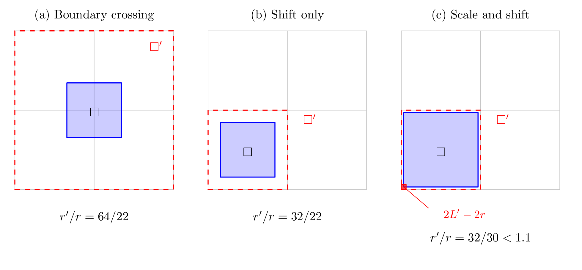
Figure 3.1: Shifting and scaling for tight containment. The shaded red patch in (c) gives admissible lower-left corners within one grid cell.

<a id="lemma31"></a>

**Lemma 3.1.** <a id="x1-15003"></a><a id="x1-150021"></a> *For a square* $`\widehat {{\square}} \in {{\mathcal{G}}}_{\mathcal{S}}`$*, and a parameter* $`{\varepsilon}\in (0,1/2)`$*, consider its randomly scaled and shifted copy* $`{\square}= \mathsf{s_r}\widehat {{\square}} + \mathsf{u_r}`$*, and its canonized version* $`{\square}' = \operatorname{canon}\left({{\square}}\right)`$*.*

*The probability that* $`r = {\mathsf{r}}\left({{\square}}\right) \leq {\mathsf{r}}\left({{\square}'}\right) \leq (1+{\varepsilon})r`$ *is* $`\geq ({\varepsilon}/8)^3`$*.*

<a id="proof1"></a>

*Proof:* <a id="x1-15005"></a>By construction $`{\square}\subseteq {\square}'`$. Let $`\ell = {\mathsf{r}}\left({\smash {\widehat {{\square}}}}\right)`$, and let $`L = 2^{\left\lceil {\log _2 \ell } \right\rceil}`$ be the rounding up of $`\ell`$ to its closest power of $`2`$, so that $`\ell \leq L < 2\ell`$. Since $`\widehat {{\square}} \subseteq [0,1/8]^2`$, we have $`\ell \leq 1/16`$ and $`L \leq 1/16`$.

The radius $`r = {\mathsf{r}}\left({{\square}}\right) = \mathsf{s_r}\ell`$ of the scaled square is uniformly distributed in $`[\ell , 2\ell ]`$. Let $`J = [(1-{\varepsilon}/4)L, (1-{\varepsilon}/8)L]`$ and $`2J = [(1-{\varepsilon}/4)2L, (1-{\varepsilon}/8)2L]`$. For an interval $`J'`$, let $`\left\|J'\right\|`$ denote its length. We have $`\left\|J\right\| = ({\varepsilon}/8)L \geq ({\varepsilon}/8)\ell`$. The two intervals are disjoint, as $`(1-{\varepsilon}/4)2L > L`$, and $`J \subseteq [\ell /2, 2\ell ]`$, as $`(1-{\varepsilon}/4)L \geq \ell /2`$ and $`L < 2\ell`$. We consider the random scaling $`\mathsf{s_r}`$ to be *good* if $`r \in J \cup 2J`$. Since $`2J \cap [\ell ,2\ell ] = 2 \left({J \cap [\ell /2, \ell ]}\right)`$, we have

```math
\left\|J \cap [\ell ,2\ell ]\right\| + \left\|2J \cap [\ell ,2\ell ]\right\| = \left\|J \cap [\ell ,2\ell ]\right\| + 2 \left\|J \cap [\ell /2,\ell ]\right\| \geq \left\|J \cap [\ell /2, 2\ell ]\right\| = \left\|J\right\| \geq ({\varepsilon}/8) \ell .
```

Thus, the random scaling is good with probability $`\geq {\varepsilon}/8`$, and assume this happened. Let $`L' = L`$ if $`r \in J`$, and $`L' = 2L`$ if $`r \in 2J`$. In either case $`L'`$ is a power of two, $`L' \leq 1/8`$, and $`2r \in [(1-{\varepsilon}/4)2L', (1-{\varepsilon}/8)2L']`$.

Consider the canonical grid $`{\mathsf{G}}_{2L'}`$. The set of all good translations

```math
U = \left\{  (x,y) \in \mathbb{R}^2  \;\middle\vert\;  (x,y) + \mathsf{s_r}\widehat {{\square}} \text { contained in a cell of } {\mathsf{G}}_{2L'}  \right\}
```

is a grid like set with sidelength $`2L'`$, where each grid point is replaced by a square of sidelength $`2L' - 2r \geq ({\varepsilon}/8)2L'`$. As $`2L' \leq 1/4`$ is a power of two, the square $`[0,1/2]^2`$ is tiled by cells of $`{\mathsf{G}}_{2L'}`$, and the probability that the random shifting $`\mathsf{u_r}`$ falls in $`U`$ is at least $`({\varepsilon}/8)^2`$.

If both things happen, then $`{\square}`$ is contained in a cell of $`{\mathsf{G}}_{2L'}`$. This cell is a canonical square, as $`{\square}\subseteq [0,3/4]^2`$ and $`2L' \leq 1/4`$, so the cell lies in $`[0,1)^2`$. Thus $`r \leq {\mathsf{r}}\left({{\square}'}\right) \leq L' \leq (1+{\varepsilon})(1-{\varepsilon}/4)L' \leq (1+{\varepsilon}) r`$. Namely, $`{\square}\subseteq {\square}'`$, and $`r = {\mathsf{r}}\left({{\square}}\right) \leq {\mathsf{r}}\left({{\square}'}\right) \leq (1+{\varepsilon})r`$, as desired.

<a id="definition32"></a>

Definition 3.2. <a id="x1-15007"></a><a id="x1-150062"></a>For a compressed quadtree $`{\mathcal{T}}`$, let $`\mathrm {cells}({\mathcal{T}})`$ be the set of all squares formed by nodes of $`{\mathcal{T}}`$. The **congestion** of a quadtree $`{\mathcal{T}}`$ for a set of segments $`{\mathcal{S}}`$ is the quantity $`{\mathit{c}}_{{\mathcal{S}}}^{}\left({{\mathcal{T}}}\right) = {\mathit{c}}_{{\mathcal{S}}}^{}\left({\mathrm {cells}({\mathcal{T}})}\right)`$.

<a id="lemma33"></a>

**Lemma 3.3.** <a id="x1-15009"></a><a id="x1-150083"></a>*Given a set* $`{\mathcal{S}}`$ *of* $`n`$ *segments, one can compute, in* $`O(n \log ^2 n)`$ *time,* $`m = O( \log n)`$ *(shifted) compressed quadtrees,* $`{\mathcal{T}}_1, \ldots , {\mathcal{T}}_m`$*, such that* $`\frac {1}{7} {\mathit{c}}\left({{\mathcal{S}}}\right)\leq \max _{i} {\mathit{c}}_{{\mathcal{S}}}^{}\left({{\mathcal{T}}_i}\right) \leq {\mathit{c}}\left({{\mathcal{S}}}\right).`$ *This holds with high probability.*

<a id="proof2"></a>

*Proof:* <a id="x1-15011"></a>Let $`{\varepsilon}\in (0,1)`$ be a sufficiently small constant to be specified shortly. Compute the set $`{{\mathcal{G}}}_{\mathcal{S}}`$ of squares specified by [Lemma 2.6](#x1-130076). Next, compute $`m = O( {\varepsilon}^{-3} \log n )`$ randomly shifted copies $`{{\mathcal{G}}}_{\mathcal{S}}^1, \ldots , {{\mathcal{G}}}_{\mathcal{S}}^m`$ of $`{{\mathcal{G}}}_{\mathcal{S}}`$, as described above. For each one of them we compute a compressed quadtree. Each such compressed quadtree can be interpreted as a shifted compressed quadtree over the original set of squares $`{{\mathcal{G}}}_{\mathcal{S}}`$. Let $`{\mathcal{T}}_1, \ldots , {\mathcal{T}}_m`$ be these quadtrees.

Fix a square $`{\square}\in {{\mathcal{G}}}_{\mathcal{S}}`$. By [Lemma 3.1](#x1-150021), with probability $`{\varsigma}\geq ({\varepsilon}/8)^3`$, there is a node $`u`$, and thus its cell $`{\square}'`$, such that $`{\square}\subseteq {\square}'`$ and $`{\mathsf{r}}\left({{\square}'}\right) \leq (1+{\varepsilon}){\mathsf{r}}\left({{\square}}\right)`$. Thus, we have $`{\mathit{c}}_{{\mathcal{S}}}^{}\left({{\square}'}\right) \geq {\mathit{c}}_{{\mathcal{S}}}^{}\left({{\square}}\right)/(1+{\varepsilon})`$.

In particular, the probability that this “good” containment does not happen for $`{\square}`$, in all $`m`$ quadtrees, is $`(1-{\varsigma})^m \leq 1/n^{O(1)}`$. We conclude that, with high probability, for all squares $`{\square}\in {{\mathcal{G}}}_{\mathcal{S}}`$, there is at least one node/square, in the computed quadtrees, that tightly contains $`{\square}`$.

This readily implies that

```math
\max _{i} {\mathit{c}}_{{\mathcal{S}}}^{}\left({{\mathcal{T}}_i}\right) \geq \frac {1}{1+{\varepsilon}}\max _{{\square}\in {{\mathcal{G}}}_{\mathcal{S}}} {\mathit{c}}_{{\mathcal{S}}}^{}\left({{\square}}\right) \geq \frac {1}{(1+{\varepsilon})(6+{\varepsilon})} {\mathit{c}}\left({{\mathcal{S}}}\right) \geq \frac {1}{7} {\mathit{c}}\left({{\mathcal{S}}}\right),
```

for $`{\varepsilon}= 1/10`$.

<a id="remark34"></a>

Remark 3.4. <a id="x1-15013"></a>Throughout the algorithm, we use compressed quadtrees, rather than regular quadtrees. The use of compressed quadtrees is necessary to get an efficient runtime, but it does not affect the description of our algorithm significantly. (Intuitively, the compressed quadtree compresses paths and not cells, so one can easily ensure that all cells of interest appear in the compressed quadtree as regular cells). As such, from this point on, we use quadtree as a shorthand for a compressed quadtree, and we ignore the minor low-level technical details that arise because of the compression.

Specifically, the only issue in the algorithm where this would make a difference is in traversing down the tree and assuming that the child is exactly half the size of its parent. This can easily be fixed by working directly with the node’s own record of its dimensions.

<a id="x1-160003.2"></a><a id="first-steps-towards-approximating-the-congestion-of-a-quadtree"></a>

### 3.2  First steps towards approximating the congestion of a quadtree

Given a set $`{\mathcal{S}}`$ of $`n`$ segments and a quadtree $`{\mathcal{T}}`$ of size $`O(n)`$, we wish to compute the congestion of $`{\mathcal{T}}`$. To simplify the exposition, we assume that any shift needed is applied to the input segments, and the quadtree is thus the standard one built over $`[0,1]^2`$.

<a id="x1-170003.2.1"></a><a id="a-na-ve-exact-algorithm-for-the-congestion-of-a-quadtree"></a>

#### 3.2.1  A naïve exact algorithm for the congestion of a quadtree

At each node $`v \in {\mathcal{T}}`$, the algorithm stores a **conflict list** $`{L}\left({v}\right)`$ – a list of all the segments of $`{\mathcal{S}}`$ intersecting the cell $`{\square}_v`$ associated with $`v`$. It begins by storing $`{\mathcal{S}}`$ at the root of $`{\mathcal{T}}`$, then recursively traverses down the tree. At each parent node $`u`$, the algorithm sends the list $`{L}\left({u}\right)`$ to all its children. Each child $`v`$ finds all the segments which intersect its cell $`{\square}_v`$ and adds them to its own list. At the end of this process, the algorithm has computed the segments intersecting each quadtree node, and it can use them to compute the congestion. Overall, this algorithm takes $`O(n^2)`$ time.

<a id="x1-180003.2.2"></a><a id="the-long-and-the-short-of-it"></a>

#### 3.2.2  The long and the short of it

To speed up the naïve algorithm, we implement several strategies. The first is to register the segments directly in the cells at a suitable resolution of the quadtree.

<a id="definition35longshort-threshold"></a>

Definition 3.5 (long/short threshold). <a id="x1-18002"></a>Let $`{\alpha}> 0`$ be a fixed integer constant, to be specified shortly[<sup>1</sup>](#fn1x0)<a id="x1-18003f1"></a> . The parameter $`{\alpha}`$ is the **transition** constant. A segment $`{s}`$ is $`{\alpha}`$**-long** (resp., $`{\alpha}`$**-short**) for a square $`{\square}= {\square}\left({{p}, r}\right)`$ if it intersects the interior of $`{\square}`$ and $`\left\|{s}\right\| \geq {\alpha}r`$ (resp., $`\left\|{s}\right\| < {\alpha}r`$). For a square $`{\square}`$ with radius $`r`$, its set of $`{\alpha}`$-long (resp., $`{\alpha}`$-short) segments is denoted by $`{\mathcal{S}}_{\geq {\alpha}}\left({{\square}}\right)`$ (resp., $`{\mathcal{S}}_{<{\alpha}}\left({{\square}}\right)`$).

<a id="computing-a-maximal-set-of-long-segments-for-a-segment-s-see-lemmaregisterlemmaref-lemmaregister-in-this-case-the-segment-has-length-5-and-each-grid-cell-is-of-radius-05-so-the-segment-is-10long-for-all-the-cells-of-the-grid-it-intersects"></a>

![grid seg-1](assets/grid_seg-1.png) ![grid seg-2](assets/grid_seg-2.png) <a id="x1-18005r2"></a>

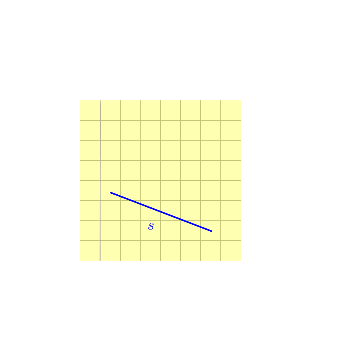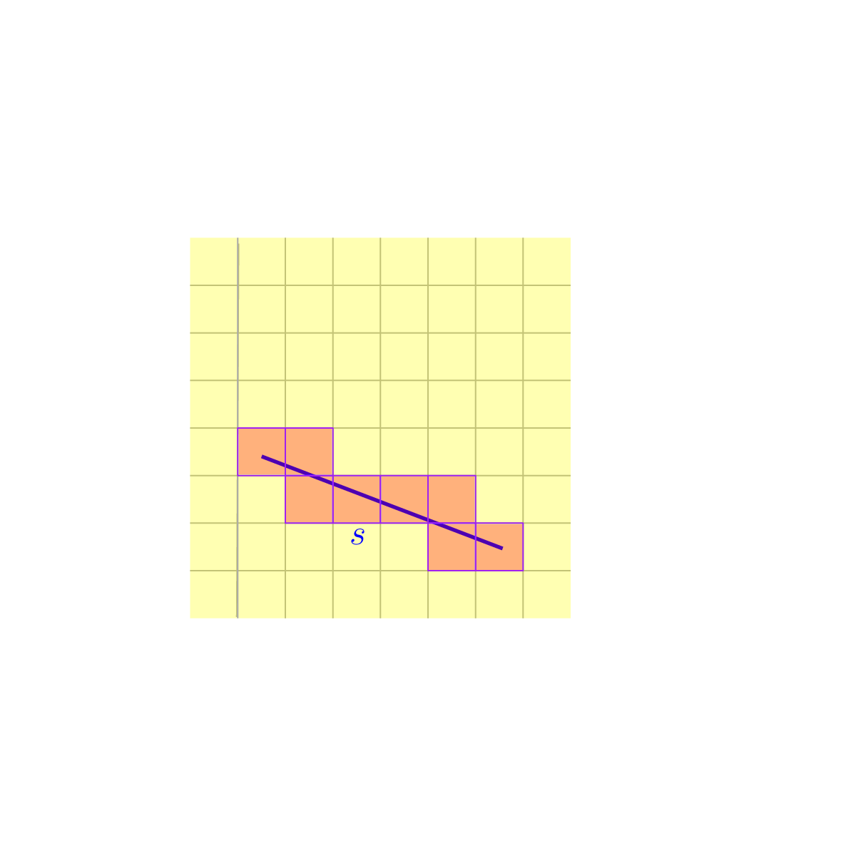
Figure 3.2: Computing a maximal set of $`{\alpha}`$-long segments for a segment $`{s}`$ (see [Lemma 3.6](#x1-180066)). In this case, the segment has length $`5`$, and each grid cell is of radius $`0.5`$, so the segment is $`10`$-long for all the cells of the grid it intersects.

<a id="lemma36"></a>

**Lemma 3.6.** <a id="x1-18007"></a><a id="x1-180066"></a>*For each segment* $`{s}\in {\mathcal{S}}`$*, let* $`{\mathsf{G}}\left({{s},{\alpha}}\right)`$ *be the set of interior-disjoint canonical squares of maximal size for which* $`{s}`$ *is* $`{\alpha}`$*-long. There are at most* $`O(1 + {\alpha})`$ *such squares, and they can be computed in* $`O(1 + {\alpha})`$ *time.*

<a id="proof3"></a>

*Proof:* <a id="x1-18009"></a>Let $`i = \left\lfloor { \log _2 (2\left\|{s}\right\|/{\alpha})} \right\rfloor`$, and $`{\tau}=2^i`$. Then

```math
\frac {{\alpha}{\tau}}{2} = {\alpha}2^{\left\lfloor {\log _2(2\left\|{s}\right\|/{\alpha})} \right\rfloor - 1} \leq \left\|{s}\right\| < {\alpha}2^{\left\lfloor {\log _2(2\left\|{s}\right\|/{\alpha})} \right\rfloor} ={\alpha}{\tau}.
```

A cell of $`{\mathsf{G}}_{\tau}`$ has radius $`{\tau}/2`$, and a canonical square of sidelength $`\geq 2{\tau}`$ has radius $`\geq {\tau}`$. Thus, $`{s}`$ is $`{\alpha}`$-long for every cell of $`{\mathsf{G}}_{\tau}`$ whose interior it intersects, but it is not $`{\alpha}`$-long for any larger canonical square. Since every canonical square of sidelength $`\leq {\tau}`$ is contained in a cell of $`{\mathsf{G}}_{\tau}`$, the set $`{\mathsf{G}}\left({{s},{\alpha}}\right)`$ is exactly the set of cells of $`{\mathsf{G}}_{\tau}`$ whose interior $`{s}`$ intersects. As $`\left\|{s}\right\| < {\alpha}{\tau}`$, the segment $`{s}`$ crosses at most $`{\alpha}`$ horizontal lines and at most $`{\alpha}`$ vertical lines of $`{\mathsf{G}}_{\tau}`$. This implies that $`{s}`$ can intersect at most $`2{\alpha}+1`$ grid cells of $`{\mathsf{G}}_{\tau}`$. Computing the grid cells that intersect $`{s}`$ is a classical problem in graphics (i.e., [line drawing problem](https://en.wikipedia.org/wiki/Line_drawing_algorithm)) which can be solved in $`O(1+{\alpha})`$ time; see [Figure 3.2](#computing-a-maximal-set-of-long-segments-for-a-segment-s-see-lemmaregisterlemmaref-lemmaregister-in-this-case-the-segment-has-length-5-and-each-grid-cell-is-of-radius-05-so-the-segment-is-10long-for-all-the-cells-of-the-grid-it-intersects).

<a id="x1-190003.2.3"></a><a id="registering-the-segments"></a>

#### 3.2.3  Registering the segments

<a id="the-refined-quadtree-t"></a> <a id="x1-20000"></a>**The refined quadtree** $`{\mathcal{T}^+}`$**.** <a id="x1-20000doc"></a> Given the set $`{\mathcal{S}}`$ of $`n`$ segments and the above quadtree $`{\mathcal{T}}`$, the algorithm first computes the set of canonical squares $`{\Xi}= \mathrm {cells}({\mathcal{T}}) \cup \bigcup _{{s}\in {\mathcal{S}}} {\mathsf{G}}\left({{s},{\alpha}}\right)`$; see [Lemma 3.6](#x1-180066). The algorithm then computes the (compressed) quadtree $`{\mathcal{T}^+}`$ for $`{\Xi}`$. This can be done in $`O( n \log n)`$ time \[[Har11](#Xh-gaa-11)\], as $`\left| {{\mathcal{S}}} \right| = n`$, $`\left| {\mathrm {cells}({\mathcal{T}})} \right| = O(n)`$, and $`\left| {{\Xi}} \right| = O( ( 1+ {\alpha}) n ) = O(n)`$, as $`{\alpha}`$ is a constant. Each square of $`{\Xi}`$ is now present as a cell of a node of the computed quadtree.

The algorithm now stores every segment $`{s}\in {\mathcal{S}}`$ in the cells of $`{\mathsf{G}}\left({{s},{\alpha}}\right)`$. Each cell $`{\square}\in {\mathsf{G}}\left({{s},{\alpha}}\right)`$ corresponds to a node $`v`$ in the quadtree, and the algorithm stores $`{s}`$ in $`{L_{\mathrm{long}}}\left({v}\right)`$. This takes $`O(n \log n)`$ time; see \[[Har11](#Xh-gaa-11)\]. Thus, for every quadtree node $`v`$, the algorithm computes a list $`{L_{\mathrm{long}}}\left({v}\right)`$ of segments registered there. Segments registered in this list are long for the cell $`{\square}_v`$ but short for cells in higher levels of the quadtree.

A segment $`{s}`$ is $`{\alpha}`$-short for the cell of every proper ancestor of a node of $`{\mathsf{G}}\left({{s},{\alpha}}\right)`$. Indeed, such a cell has radius at least the sidelength $`{\tau}`$ of the cells of $`{\mathsf{G}}\left({{s},{\alpha}}\right)`$, while $`\left\|{s}\right\| < {\alpha}{\tau}`$, see the proof of [Lemma 3.6](#x1-180066). As such, the lists $`{L_{\mathrm{long}}}\left({\cdot }\right)`$ also determine the short segments of every node, see [Definition 3.7](#x1-200027), and no separate registration of short segments is needed. The lists $`{L_{\mathrm{long}}}\left({\cdot }\right)`$ have total length $`O(n)`$.

A segment is registered only once on any path in the quadtree, as the cells of $`{\mathsf{G}}\left({{s},{\alpha}}\right)`$ are interior disjoint; see [Figure 3.3](#long-lists-propagate-downward-short-clipped-lengths-accumulate-upward-the-two-registered-pieces-of-t-contribute-once-each).

<a id="long-lists-propagate-downward-short-clipped-lengths-accumulate-upward-the-two-registered-pieces-of-t-contribute-once-each"></a>

![long short flow-](assets/long_short_flow-.png) <a id="x1-20001r3"></a>

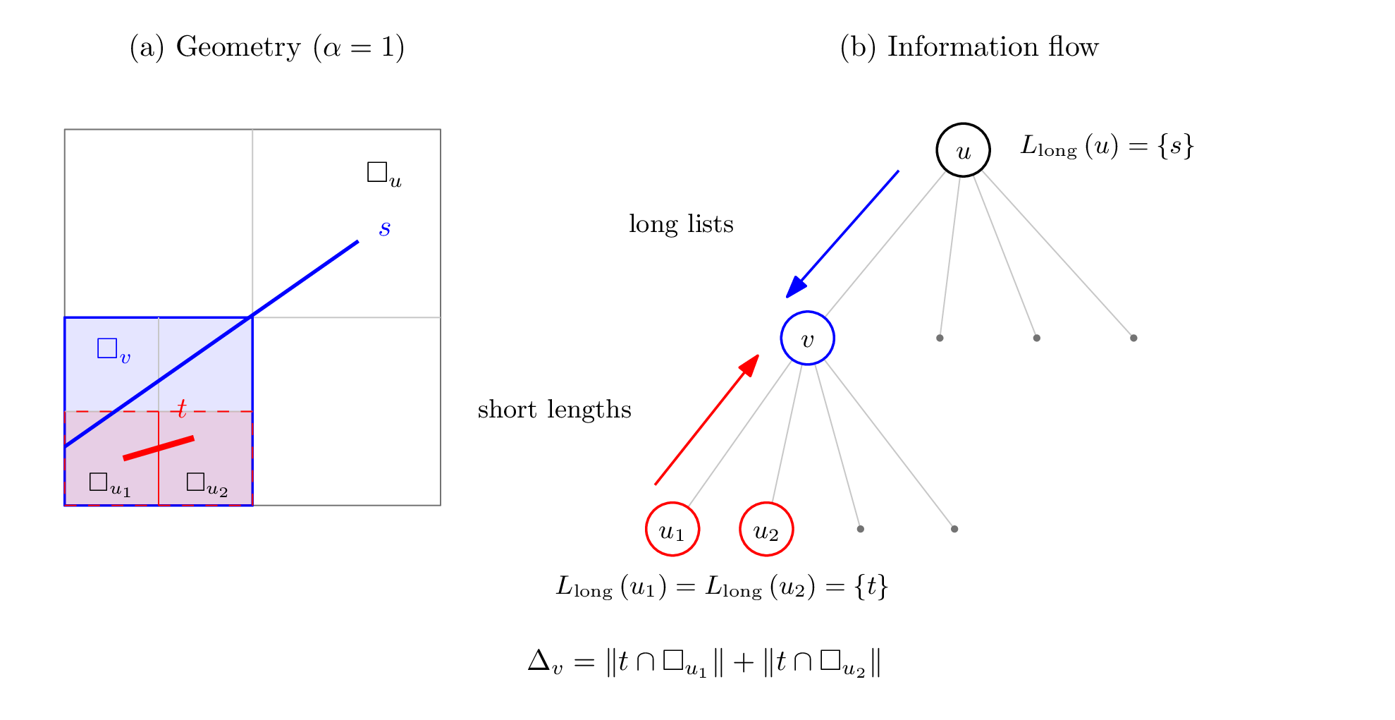
Figure 3.3: Long lists propagate downward; short clipped lengths accumulate upward. The two registered pieces of $`t`$ contribute once each.

<a id="definition37"></a>

Definition 3.7. <a id="x1-20003"></a><a id="x1-200027"></a>For a node $`v \in {\mathcal{T}^+}`$, let $`\mathrm{anc}\left({v}\right)`$ (resp., $`\mathrm{desc}\left({v}\right)`$) be the list of ancestors (resp., descendants) of $`v`$ in the tree $`{\mathcal{T}^+}`$. By convention, $`v \in \mathrm{anc}\left({v}\right)`$ and $`v \in \mathrm{desc}\left({v}\right)`$, that is, a node is its own ancestor and descendant. Consider a node $`v \in {\mathcal{T}^+}`$, and let $`{\square}_v`$ be its associated square. We have that

```math
{\mathcal{S}}_{\geq {\alpha}}\left({{\square}_v}\right)=\bigcup _{u \in \mathrm{anc}\left({v}\right)} \left({{L_{\mathrm{long}}}\left({u}\right) \cap {\square}_v}\right) \qquad \text {and}\qquad {\mathcal{S}}_{<{\alpha}}\left({{\square}_v}\right)=\bigcup _{u \in \mathrm{desc}\left({v}\right) \setminus \{v\}} {L_{\mathrm{long}}}\left({u}\right).
```

<a id="definition38"></a>

Definition 3.8. <a id="x1-20005"></a><a id="x1-200048"></a>The $`{\alpha}`$**-long congestion** of $`{\square}`$ is $`{\mathit{c}}^{}_{\!\hspace{0.6pt}\geq {\alpha}}\left({{\square}}\right) = \left\| {\mathcal{S}}_{\geq {\alpha}}\left({{\square}}\right) \sqcap {\square}\right\|/r`$. Similarly the $`{\alpha}`$**-short congestion** of $`{\square}`$ is $`{\mathit{c}}_{<{\alpha}}\left({{\square}}\right) = \left\|{\mathcal{S}}_{<{\alpha}}\left({{\square}}\right) \sqcap {\square}\right\|/r`$. Given a quadtree $`{\mathcal{T}}`$, its $`{\alpha}`$**-long congestion** and $`{\alpha}`$**-short congestion** are

```math
{\mathit{c}}^{}_{\!\hspace{0.6pt}\geq {\alpha}}= {\mathit{c}}^{}_{\!\hspace{0.6pt}\geq {\alpha}}\left({{\mathcal{T}}}\right) = \max _{{\square}\in \mathrm {cells}({\mathcal{T}})} {\mathit{c}}^{}_{\!\hspace{0.6pt}\geq {\alpha}}\left({{\square}}\right) \qquad \text {and}\qquad {\mathit{c}}_{<{\alpha}}= {\mathit{c}}_{<{\alpha}}\left({{\mathcal{T}}}\right) = \max _{{\square}\in \mathrm {cells}({\mathcal{T}})} {\mathit{c}}_{<{\alpha}}\left({{\square}}\right).
```

To summarize, we have described how to augment a quadtree $`{\mathcal{T}}`$ by adding more cells and registering the segments at the cells, yielding a new quadtree $`{\mathcal{T}^+}`$. In what follows, we use this stored information to compute the long and short congestions of $`{\mathcal{T}^+}`$ (which are at least the congestions of the sub-quadtree $`{\mathcal{T}}`$).

<a id="x1-210003.3"></a><a id="computing-the-congestion-of-the-short-segments"></a>

### 3.3  Computing the congestion of the short segments

The $`{\alpha}`$-short congestion is computed using dynamic programming, as described next.

<a id="lemma39"></a>

**Lemma 3.9.** <a id="x1-21002"></a><a id="x1-210019"></a>*Given a set* $`{\mathcal{S}}`$ *of* $`n`$ *segments in the plane and a quadtree* $`{\mathcal{T}^+}`$ *of size* $`O(n)`$*, one can compute, in* $`O(n )`$ *time, the* $`{\alpha}`$*-short congestion for all the nodes of* $`{\mathcal{T}^+}`$*, where* $`{\alpha}`$ *is a constant.*

<a id="proof4"></a>

*Proof:* <a id="x1-21004"></a>We compute the $`{\alpha}`$-short congestion of a quadtree via dynamic programming. The algorithm finds the total length of short segments intersecting each leaf and propagates the values upward.

For every node $`v \in {\mathcal{T}^+}`$, the algorithm computes the quantity $`\left\|{L_{\mathrm{long}}}\left({v}\right) \sqcap {\square}_v\right\|`$. Computing the value for node $`v`$ requires time proportional to the total size of the list $`{L_{\mathrm{long}}}\left({v}\right)`$, so doing it for all the nodes of the tree takes $`O(n)`$ time overall. Next, the algorithm traverses the tree bottom-up. For each node along the way, it computes the total lengths of the intersecting short segments, summing over the proper descendants of $`v`$:

```math
{\Delta}_{v}=\sum _{u \in \mathrm{desc}\left({v}\right) \setminus \{v\}} \left\|{L_{\mathrm{long}}}\left({u}\right) \sqcap {\square}_u\right\| =\sum _{u \text { child of }v} \left({ \left\|{L_{\mathrm{long}}}\left({u}\right) \sqcap {\square}_u\right\| + {\Delta}_{u} }\right).
```

We claim that $`{\Delta}_{v} = \left\|{\mathcal{S}}_{<{\alpha}}\left({{\square}_v}\right) \sqcap {\square}_v\right\|`$. Consider a segment $`{s}\in {\mathcal{S}}_{<{\alpha}}\left({{\square}_v}\right)`$, and let $`{\tau}`$ be the sidelength of the cells of $`{\mathsf{G}}\left({{s},{\alpha}}\right)`$. By the proof of [Lemma 3.6](#x1-180066), $`{\alpha}{\tau}/2 \leq \left\|{s}\right\| < {\alpha}{\mathsf{r}}\left({{\square}_v}\right)`$, so the sidelength of $`{\square}_v`$ is at least $`2{\tau}`$, and $`{\square}_v`$ is a union of cells of $`{\mathsf{G}}_{\tau}`$. The cells of $`{\mathsf{G}}\left({{s},{\alpha}}\right)`$ contained in $`{\square}_v`$ are proper descendants of $`v`$ in $`{\mathcal{T}^+}`$, they are interior disjoint, and they cover $`{s}\cap {\square}_v`$, while the other cells of $`{\mathsf{G}}\left({{s},{\alpha}}\right)`$ are interior disjoint from $`{\square}_v`$. Thus $`{s}`$ contributes exactly $`\left\|{s}\cap {\square}_v\right\|`$ to the sum. Conversely, a segment registered at a proper descendant $`u`$ of $`v`$ is $`{\alpha}`$-short for $`{\square}_v`$, as $`{\mathsf{r}}\left({{\square}_v}\right) \geq 2 {\mathsf{r}}\left({{\square}_u}\right) > \left\|{s}\right\|/{\alpha}`$. The lemma follows.

<a id="x1-220004"></a><a id="approximating-the-maximum-load-of-the-long-segments-in-a-quadtree"></a>

## 4  Approximating the maximum load of the long segments in a quadtree

Handling the long congestion quickly seems challenging. Instead, we quickly approximate a proxy for this quantity – the maximum number of long segments intersecting a single cell.

<a id="definition41"></a>

Definition 4.1. <a id="x1-22002"></a><a id="x1-220011"></a>The $`{\alpha}`$**-load** of a quadtree $`{\mathcal{T}^+}`$ is the quantity

```math
{\rho}= \max _{{\square}\in \mathrm {cells}({\mathcal{T}^+})} |{\mathcal{S}}_{\geq {\alpha}}\left({{\square}}\right)|.
```

<a id="x1-230004.1"></a><a id="a-na-ve-algorithm-for-computing-the-load"></a>

### 4.1  A naïve algorithm for computing the $`{\alpha}`$-load

To compute the exact load of a given square, we need to find the long segments intersecting it. We can compute the conflict list for each cell by pushing long segments downward from the conflict lists of its ancestors (as done in the naïve algorithm of [Section 3.2.1](#a-na-ve-exact-algorithm-for-the-congestion-of-a-quadtree)). Unfortunately, these lists can get quite long.

<a id="lemma42"></a>

**Lemma 4.2.** <a id="x1-23002"></a><a id="x1-230012"></a>*One can compute the* $`{\alpha}`$*-load of* $`{\mathcal{T}^+}`$ *in* $`O(n \log n + {\rho}n )`$ *time. More generally, given a set* $`{R}\subseteq {\mathcal{S}}`$ *and a threshold* $`t`$*, one can decide whether* $`{\rho}\left({{R}}\right) = \max _{{\square}\in \mathrm {cells}({\mathcal{T}^+})} |{R}\cap {\mathcal{S}}_{\geq {\alpha}}\left({{\square}}\right)| \leq t`$*, in* $`O(n \log n + t n)`$ *time.*

<a id="proof5"></a>

*Proof:* <a id="x1-23004"></a>The algorithm starts with the precomputed lists $`{L_{\mathrm{long}}}\left({u}\right)`$ and traverses the tree top-down. At each node, it pushes the stored list down to the children. Each child $`v`$ selects the segments of the incoming list that intersect its cell, and takes the union of this filtered incoming list with $`{L_{\mathrm{long}}}\left({v}\right)`$. This yields the conflict list of $`v`$ of *all* $`{\alpha}`$-long segments that intersect it, denoted by $`{L_{\mathrm{LONG}}}\left({v}\right)`$. It then pushes this list down to its children, and so on.

For each node $`v`$ of the quadtree, it is now straightforward to compute the congestion of the segments of $`{L_{\mathrm{LONG}}}\left({v}\right)`$ (or the length of the list $`{L_{\mathrm{LONG}}}\left({v}\right)`$) for the cell of the node $`v`$. It follows that this computes the $`{\alpha}`$-long congestion for each node of the quadtree. Since the maximum length of the lists sent down is $`{\rho}`$, the claim follows.

The second algorithm works in a similar fashion, except that the algorithm propagates downwards only segments of $`{R}`$. If in any point in time the computed conflict list gets bigger than $`t`$, the algorithm bails out, returning that $`{\rho}\left({{R}}\right) > t`$.

<a id="x1-23005r1"></a>

<a id="an-long-segment-for-a-square-p-r-intersects-the-square-p-1-r-with-a-segment-of-length-at-least-r-here-3"></a>

![enlarge-](assets/enlarge-.png)

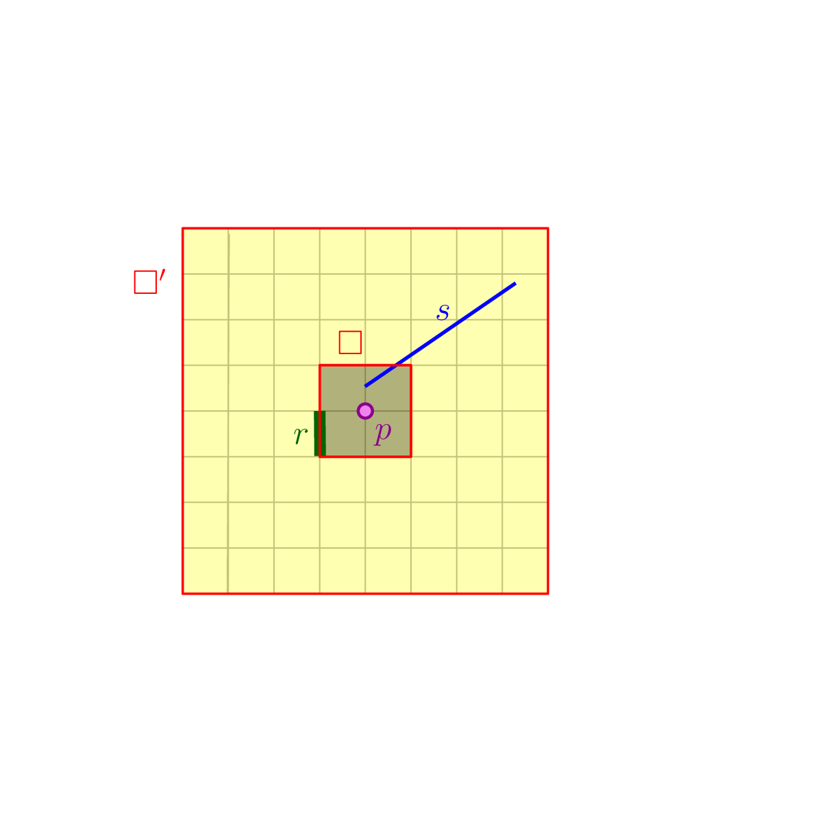
Figure 4.1: An $`{\alpha}`$-long segment for a square $`{\square}= {\square}\left({{p}, r}\right)`$ intersects the square $`{\square}' = {\square}\left({{p}, (1+{\alpha})r}\right)`$ with a segment of length at least $`{\alpha}r`$ (here, $`{\alpha}=3`$).

<a id="x1-240004.2"></a><a id="from-long-congestion-to-load-and-back"></a>

### 4.2  From long congestion to load, and back

Instead of computing the $`{\alpha}`$-long congestion of a quadtree exactly, we content ourselves with a constant-factor approximation, by using the load instead.

<a id="lemma43"></a>

**Lemma 4.3.** <a id="x1-24002"></a><a id="x1-240013"></a>*For a cell* $`{\square}= {\square}\left({{p}, r}\right)`$ *of* $`{\mathcal{T}^+}`$*, we have* $`\displaystyle \frac {{\mathit{c}}^{}_{\!\hspace{0.6pt}\geq {\alpha}}\left({{\square}}\right)}{\sqrt {8}}\leq |{\mathcal{S}}_{\geq {\alpha}}\left({{\square}}\right)|\leq \frac {1+{\alpha}}{{\alpha}} {\mathit{c}}\left({{\mathcal{S}}}\right).`$

<a id="proof6"></a>

*Proof:* <a id="x1-24004"></a>The intersection of each segment of $`{\mathcal{S}}_{\geq {\alpha}}\left({{\square}}\right)`$ with $`{\square}`$ can have length at most $`\sqrt {2}\cdot 2 r = \sqrt {8}r`$ (as the sidelength of $`{\square}`$ is $`2r`$), so $`{\mathit{c}}^{}_{\!\hspace{0.6pt}\geq {\alpha}}\left({{\square}}\right) = \left\| {\mathcal{S}}_{\geq {\alpha}}\left({{\square}}\right) \sqcap {\square}\right\|/ r`$, and $`\left\| {\mathcal{S}}_{\geq {\alpha}}\left({{\square}}\right) \sqcap {\square}\right\|\leq |{\mathcal{S}}_{\geq {\alpha}}\left({{\square}}\right)| \cdot r \sqrt {8}`$, and the first inequality follows.

As for the second inequality, consider $`{\square}' = {\square}\left({{p}, (1+{\alpha})r}\right)`$. By definition, each long segment $`{s}\in {\mathcal{S}}_{\geq {\alpha}}\left({{\square}}\right)`$ has length at least $`{\alpha}r`$ and intersects $`{\square}`$. The length of $`{s}\cap {\square}'`$ is at least $`{\alpha}r`$, see [Figure 4.1](#an-long-segment-for-a-square-p-r-intersects-the-square-p-1-r-with-a-segment-of-length-at-least-r-here-3). As such, we have

```math
\left| {{\mathcal{S}}_{\geq {\alpha}}\left({{\square}}\right)} \right| \cdot \frac {{\alpha}r}{(1+{\alpha})r} \leq \frac {\left\|{\mathcal{S}}_{\geq {\alpha}}\left({{\square}}\right) \sqcap {\square}'\right\|}{(1+{\alpha})r}\leq {\mathit{c}}\left({{\square}'}\right) \leq {\mathit{c}}\left({{\mathcal{S}}}\right).
```

<a id="x1-250004.3"></a><a id="exponential-search-for-maximum-load"></a>

### 4.3  Exponential search for maximum $`{\alpha}`$-load

It remains to estimate the load (i.e., maximum number of $`{\alpha}`$-long segments intersecting any cell in the quadtree $`{\mathcal{T}^+}`$). The basic idea is to couple random sampling together with exponential search, to approximate the maximum load. If during a round an “overflow” occurs, the algorithm increases the guess for the load (say, by a factor of $`2`$), and moves on to the next round. Using sampling and exponential search to estimate a quantity is an old idea. In the context of geometric settings, it was used before to estimate the maximum depth of nicely behaved regions, see Aronov and Har-Peled \[[AH08](#Xah-adrp-08)\].

<a id="x1-260004.3.1"></a><a id="the-algorithm"></a>

#### 4.3.1  The algorithm

Our purpose here is to approximate the $`{\alpha}`$-load of $`{\mathcal{T}^+}`$, denoted by $`{\rho}`$, see [Definition 4.1](#x1-220011).

<a id="estimation-via-sampling"></a> <a id="x1-27000"></a>**Estimation via sampling.** We perform an exponential search for the size of the largest conflict list. We use the following standard sampling lemma. It follows by a standard application of Chernoff’s inequality – see Beame *et al.* \[[BHR<sup>+</sup>20](#Xbhrrs-eeiso-20), Lemma 2.7\] for a proof.

<a id="lemma44"></a>

**Lemma 4.4.** <a id="x1-27002"></a><a id="x1-270014"></a>*Consider two (finite) sets* $`B\subseteq \mathcal{S}`$*, where* $`n = \left| {\mathcal{S}} \right|`$*. Let* $`{\xi}\in (0,1)`$ *and* $`\varphi\in (0,1/2)`$ *be parameters, and let* $`r = \left\lceil {\smash {c_2{\xi}^{-2} \tfrac {n}{g} \log \varphi^{-1}}\bigr .} \right\rceil`$*, where* $`c_2`$ *is a sufficiently large constant.*

*Let* $`g > 0`$ *be a user-provided guess for the size of* $`\left| {B} \right|`$*. Consider a random sample* $`{R}`$*, taken from* $`\mathcal{S}`$ *by picking each element with probability* $`\tfrac {r}{n}`$*. Next, consider the estimate* $`Y = \tfrac {n}{r} \left| { {R}\cap B} \right|`$ *to* $`\left| {B} \right|`$*. Then, we have the following:*

- **(A)** *If* $`Y < g/2`$*, then* $`\left| {B} \right| < g`$*,*
- **(B)** *If* $`Y \geq g/2`$*, then* $`(1-{\xi})Y \leq \left| {B} \right| \leq (1+{\xi})Y`$*.*

*Both statements above hold with probability* $`\geq 1-\varphi`$*.*

<a id="the-algorithm1"></a> <a id="x1-28000"></a>**The algorithm.** The number of cells in $`{\mathcal{T}^+}`$ is $`O(n)`$, and let $`\varphi=1/n^{O(1)}`$. Let $`{\varepsilon}\in (0,1)`$ be a prespecified approximation parameter, and let $`{\xi}= {\varepsilon}/3`$. At each round, the algorithm has a threshold number $`g_i`$ and checks whether (i) $`{\rho}> 8g_i`$ (roughly), or (ii) $`{\rho}=\Theta (g_i)`$ and it can be approximated reliably and quickly. The $`i`$th round starts with parameters <a id="x1-28001r1"></a>

```math
g_i = 2^{i-1} \qquad \text {and}\qquad r_i = \left\lceil {\smash {c_2{\xi}^{-2} \tfrac {n}{g_i} \log \varphi^{-1}}} \right\rceil,  \tag{4.1}
```

where $`c_2`$ is a sufficiently large constant. If the $`i`$th round failed, the algorithm goes on to the next round (i.e., by increasing $`i`$ by one).

Let $`I`$ be the first integer such that $`r_i < n`$ (i.e., $`g_I = \Theta ( {\xi}^{-2} \log n )`$ and $`I = O( \log \log n + \log {\varepsilon}^{-1})`$), and the algorithm starts with $`i=I`$. In this first round, the algorithm uses [Lemma 4.2](#x1-230012) directly. If it finds some conflict list (for $`{\mathcal{S}}`$) that contains more than $`8g^{}_i = 8 g_I^{}`$ segments at any point during the execution, it concludes that $`g_i`$ is too small. Thus this round is a failure, and it goes on to the next round. Otherwise, the algorithm computes $`{\rho}`$ exactly and returns its value.

For later rounds, and larger values of $`g_i`$, the round begins by taking a random sample $`{R}_i \subseteq {\mathcal{S}}`$ of the segments. Each segment is included in $`{R}_i`$ independently with probability $`{\varsigma}_i= r_i / n`$ (i.e., a random sample according to [Lemma 4.4](#x1-270014)). The algorithm then calls the subroutine of [Lemma 4.2](#x1-230012) with $`{R}_i`$ as the list of segments and with $`U_i = 8 g_i {\varsigma}_i`$ as the threshold. If the output reveals that $`{\rho}\left({{R}_i}\right) > U_i`$, then the guess $`g_i`$ is too small, the round failed, and the algorithm continues to the next round.

If a round succeeds (and $`i \neq I`$), the algorithm outputs $`(1-{\xi})Y`$ for $`Y= \tfrac {n}{r_i}{\rho}\left({{R}_i}\right)`$ as an estimate from below to $`{\rho}`$.

<a id="x1-290004.3.2"></a><a id="analysis"></a>

#### 4.3.2  Analysis

<a id="running-time"></a> <a id="x1-30000"></a>**Running time.** The first round takes $`O( {\varepsilon}^{-2} n\log n )`$ time. Since there are only $`n`$ segments in $`{\mathcal{S}}`$, the algorithm always stops by round $`O( \log n)`$. The threshold used in each round is

```math
U_i =8g_i {\varsigma}_i = \frac {8g_i r_i}{n} = O\left({ \smash {\frac {g_i}{n} \cdot \frac {n}{{\xi}^2 g_i} } \log n^{O(1)} }\right) = O\Bigl ( \frac {\log n}{{\varepsilon}^{2}} \Bigr ).
```

As such, the running time of each round is $`O({\varepsilon}^{-2} n \log n)`$; see [Lemma 4.2](#x1-230012), and the overall running time is $`O({\varepsilon}^{-2} n \log ^2 n)`$.

<a id="the-result"></a> **<a id="x1-31000"></a>The result.**

<a id="lemma45"></a>

**Lemma 4.5.** <a id="x1-31002"></a><a id="x1-310015"></a>*Using the above randomized algorithm, one can compute, in* $`O( {\varepsilon}^{-2}n{\log ^2 n} )`$ *time, a number* $`\Delta`$*, such that with high probability, we have* $`\Delta \leq {\rho}\leq (1+{\varepsilon})\Delta ,`$ *where* $`{\rho}`$ *is the* $`{\alpha}`$*-load of* $`{\mathcal{T}^+}`$*, see* [Definition 4.1](#x1-220011)*.*

<a id="proof7"></a>

*Proof:* <a id="x1-31004"></a>If the algorithm terminated after the first round, then it output $`{\rho}`$ exactly, and we are done.

Otherwise, if it failed in a round, it must be that it found a node whose conflict list exceeds the “expected” threshold $`U_i = 8 g_i {\varsigma}_i`$. [Lemma 4.4](#x1-270014) implies that the random sample in such cases estimates the size of the original conflict list correctly (its estimate $`Y`$ exceeds $`(n/r_i) U_i = 8 g_i \geq g_i/2`$), and it is at least of size $`(1-{\xi})8 g_i > 4 g_i`$. Namely, $`g_i`$ is (way) too small, and this decision was made correctly with probability $`1 - 1/n^{O(1)}`$.

If the algorithm succeeded in a round, then [Lemma 4.4](#x1-270014) implies that $`{\rho}\leq (1+{\xi})8 g_i < 16 g_i`$, as every estimate is at most $`(n/r_i)U_i = 8g_i`$. Since the algorithm failed the previous round, we have that $`{\rho}> 4g_{i-1} \geq 2g_i`$. [Lemma 4.4](#x1-270014) then implies that $`{\rho}`$ is $`(1\pm {\xi})`$-estimated correctly. Specifically, for the $`j`$th “heavy” node (i.e., conflict list size $`{\rho}_j`$ is larger than $`g_i`$) in the tree, let $`Y_j`$ be the estimate of its conflict list size. We have that $`(1-{\xi})Y_j \leq {\rho}_j \leq (1+{\xi})Y_j`$. This inequality clearly holds also on the max value, which implies that

```math
(1-{\xi})Y \leq {\rho}\leq (1+{\xi})Y \implies \Delta = (1-{\xi})Y \leq {\rho}\leq \frac {1+{\xi}}{1-{\xi}}\Delta \leq (1+ 3{\xi})\Delta = (1+{\varepsilon})\Delta ,
```

as $`{\xi}= {\varepsilon}/3 < 1/3`$.

An important technicality here is that any of the conflict lists in the tree of size smaller than $`g_i/2`$ are too small after the sampling to compete with the conflict list realizing $`{\rho}`$. Similarly, this also holds for conflict lists of size $`\leq g_i`$. Thus, all the conflict lists in play for realizing the maximum of the sample are estimated correctly[<sup>2</sup>](#fn2x0)<a id="x1-31005f2"></a> .

<a id="x1-320005"></a><a id="approximating-the-maximum-congestion"></a>

## 5  Approximating the maximum congestion

We seem to have lost our way, so let us get back on track. Consider the following quantity

```math
{\mathcal{C}}^{}_{\!\hspace{0.6pt}\geq {\alpha}}({\mathcal{T}^+}) = \max _{{\square}\in \mathrm {cells}({\mathcal{T}^+})} \max \bigl [ {\mathit{c}}^{}_{\!\hspace{0.6pt}\geq {\alpha}}\left({{\square}}\right), {\mathit{c}}_{{\mathcal{S}}_{\geq {\alpha}}\left({{\square}}\right)}^{}\left({(1+{\alpha}){\square}\bigr .}\right)\bigr ],
```

which is the **augmented** long congestion of $`{\mathcal{T}^+}`$. We define[<sup>3</sup>](#fn3x0)<a id="x1-32001f3"></a>

```math
{\mathcal{C}}_{{\mathcal{S}}}^{}\left({{\mathcal{T}^+}}\right) = \max \left({ {\mathit{c}}_{<{\alpha}}({\mathcal{T}^+}), {\mathcal{C}}^{}_{\!\hspace{0.6pt}\geq {\alpha}}({\mathcal{T}^+})}\right).
```

Clearly, $`{\mathit{c}}_{{\mathcal{S}}}^{}\left({{\mathcal{T}^+}}\right)/2 \leq {\mathcal{C}}_{{\mathcal{S}}}^{}\left({{\mathcal{T}^+}}\right) \leq {\mathit{c}}\left({{\mathcal{S}}}\right)`$.

<a id="lemma51"></a>

**Lemma 5.1.** <a id="x1-32004"></a><a id="x1-320031"></a>*We have* $`\frac {{\alpha}}{1+{\alpha}} {\rho}\leq {\mathcal{C}}^{}_{\!\hspace{0.6pt}\geq {\alpha}}({\mathcal{T}^+}) \leq \sqrt {8} {\rho}`$*.*

<a id="proof8"></a>

*Proof:* <a id="x1-32006"></a>The upper bound is immediate. The lower bound readily follows from the argument used in the proof of [Lemma 4.3](#x1-240013).

<a id="lemma52"></a>

**Lemma 5.2.** <a id="x1-32008"></a><a id="x1-320072"></a>*One can compute, in* $`O(n \log ^2 n)`$ *time, a quantity* $`\mathcal{A}_{{\mathcal{S}}}^{}\left({{\mathcal{T}^+}}\right),`$ *such that* $`\mathcal{A}_{{\mathcal{S}}}^{}\left({{\mathcal{T}^+}}\right) \leq {\mathcal{C}}_{{\mathcal{S}}}^{}\left({{\mathcal{T}^+}}\right) \leq 3 \mathcal{A}_{{\mathcal{S}}}^{}\left({{\mathcal{T}^+}}\right).`$ *This holds with high probability.*

<a id="proof9"></a>

*Proof:* <a id="x1-32010"></a>Let $`{\varepsilon}= 1/100`$, and let $`\Delta`$ be the approximation of $`{\rho}`$ computed by the algorithm of [Lemma 4.5](#x1-310015). This takes $`O(n \log ^2 n )`$ time. We now compute $`{\mathit{c}}_{<{\alpha}}({\mathcal{T}^+})`$ in $`O(n)`$ time using the algorithm of [Lemma 3.9](#x1-210019). We compute the quantity

```math
\mathcal{A}_{{\mathcal{S}}}^{}\left({{\mathcal{T}^+}}\right) = \max \Bigl ( {\mathit{c}}_{<{\alpha}}({\mathcal{T}^+}), \frac {{\alpha}}{1+{\alpha}}\Delta \Bigr ).
```

Clearly, $`\mathcal{A}_{{\mathcal{S}}}^{}\left({{\mathcal{T}^+}}\right) \leq {\mathcal{C}}_{{\mathcal{S}}}^{}\left({{\mathcal{T}^+}}\right)`$. As for the other direction, observe that

```math
\frac {\sqrt {8}(1+{\varepsilon})(1+{\alpha})}{{\alpha}} \mathcal{A}_{{\mathcal{S}}}^{}\left({{\mathcal{T}^+}}\right) \geq \frac {{\alpha}}{1+{\alpha}}\Delta \cdot \frac {\sqrt {8}(1+{\varepsilon})(1+{\alpha})}{{\alpha}} \geq \sqrt {8} {\rho}\geq {\mathcal{C}}^{}_{\!\hspace{0.6pt}\geq {\alpha}}({\mathcal{T}^+}),
```

by [Lemma 5.1](#x1-320031). Numerical calculations show that for $`{\varepsilon}=1/100`$ and $`{\alpha}=20`$, $`\frac {\sqrt {8}(1+{\varepsilon})(1+{\alpha})}{{\alpha}} \leq 3`$, which establishes the claim.

Finally, we arrive at our main result.

<a id="theorem53"></a>

**Theorem 5.3.** <a id="x1-32012"></a><a id="x1-320113"></a>*Let* $`{\mathcal{S}}`$ *be a set of* $`n`$ *segments in the plane. One can compute, in* $`O(n \log ^3 n)`$ *time, a* $`42`$*-approximation to* $`{\mathit{c}}\left({{\mathcal{S}}}\right)`$*. The algorithm is randomized and succeeds with high probability.*

<a id="proof10"></a>

*Proof:* <a id="x1-32014"></a>Compute, in $`O(n \log ^2 n)`$ time, the $`m=O(\log n)`$ quadtrees $`{\mathcal{T}}_1, \ldots , {\mathcal{T}}_m`$ of [Lemma 3.3](#x1-150083). Each quadtree $`{\mathcal{T}}_i`$ is refined as described in [Section 3.2.3](#x1-20000doc), into a quadtree $`{\mathcal{T}}_i^+`$, and we compute for each one of them the quantity $`\zeta _i = \mathcal{A}_{{\mathcal{S}}}^{}\left({{\mathcal{T}}^+_i}\right)`$, using the algorithm of [Lemma 5.2](#x1-320072) in $`O(n \log ^2 n)`$ time. Overall, the running time is $`O( n\log ^3 n )`$, and all the steps so far succeeded with high probability. The algorithm returns $`\zeta = \max _i \zeta _i \leq {\mathit{c}}\left({{\mathcal{S}}}\right)`$ as the desired approximation to the congestion. For the quality of approximation, observe that

```math
42 \zeta = 14 \max _i 3 \zeta _i \geq 14 \max _i {\mathcal{C}}_{{\mathcal{S}}}^{}\left({{\mathcal{T}}^+_i}\right) \geq 7 \max _i {\mathit{c}}_{{\mathcal{S}}}^{}\left({{\mathcal{T}}^+_i}\right) \geq 7 \cdot \frac {1}{7} {\mathit{c}}\left({{\mathcal{S}}}\right) ={\mathit{c}}\left({{\mathcal{S}}}\right).
```

<a id="x1-330006"></a><a id="a-1-approximation-in-nearlinear-time"></a>

## 6  A $`(1+{\varepsilon})`$-approximation in near-linear time

In this section we improve the approximation factor to $`1+{\varepsilon}`$, for any fixed $`{\varepsilon}>0`$, while keeping the running time near-linear. The guarantee is for the axis-parallel square congestion of [Definition 2.4](#x1-130034). Specifically, we show ([Theorem 6.7](#x1-450107)) that for a set $`{\mathcal{S}}`$ of $`n`$ segments in the plane, and any fixed $`q>0`$, one can compute a number $`A`$ with $`A\leq {\mathit{c}}\left({{\mathcal{S}}}\right)\leq (1+{\varepsilon})A`$, with probability at least $`1-(n+2)^{-q}`$, in $`O_{{\varepsilon},q}(n\log ^6(n+2))`$ time in the worst case and $`O_{{\varepsilon},q}(n\log ^5(n+2))`$ expected time.

The algorithm of the preceding sections only estimates the congestion of fixed squares, namely quadtree cells and their inflated copies, and it uses the load of a cell (a count of long segments) as a proxy for its long congestion. Here every small long-segment list is evaluated twice: clipped to its own cell, and as a free-standing input whose congestion is maximized over all squares, with center and radius unconstrained. The second evaluation is what allows us to recover an almost optimal square whose center is far from any endpoint. The section is organized as follows. We first show that the congestion of any set of $`k`$ segments is realized by one of $`O(k^3)`$ squares, so the congestion of a small list can be computed exactly ([Lemma 6.2](#x1-390012)). We then prove a sampling lemma for lengths, rather than counts, showing that a random sample of the segments has congestion close to the scaled congestion of the input, once the latter is large enough ([Lemma 6.3](#x1-400023)). Next, we describe a refined family of candidate squares, built from a well-separated pair decomposition of the endpoints, and an evaluator that computes the two values above for every cell of the quadtrees built for this family. For an accuracy parameter $`{\xi}`$, its output is a $`(1-3{\xi})`$-approximation to the congestion of its input, provided all long lists are small ([Lemma 6.6](#x1-440046)). Finally, an exponential search over sampling rates, as in [Section 4](#approximating-the-maximum-load-of-the-long-segments-in-a-quadtree), finds a sample that is dense enough to be accurate, and sparse enough for all long lists to be small ([Section 6.5](#a-simple-stopping-rule)). See [Algorithm 6.1](#x1-450011) for the resulting loop.

<a id="conventions"></a> **<a id="x1-34000"></a>Conventions.** We use the notation of [Section 2](#preliminaries). We work in the real RAM, as the preceding sections implicitly do, where arithmetic operations, square roots, the floor function, and comparisons take unit time. In particular, [Lemma 6.2](#x1-390012) is exact in this model, as the sum-of-square-roots issue mentioned in the introduction does not arise when square roots are exact. The input $`{\mathcal{S}}`$ is a multiset of segments, that is, segments count with multiplicity. We discard zero-length segments, and for an empty input the algorithm returns zero. For a single segment $`{s}`$, we write $`{\mathit{c}}_{{s}}^{}\left({{\square}}\right)=\left\|{s}\cap {\square}\right\|/{\mathsf{r}}\left({{\square}}\right)`$. A segment meets a square $`{\square}`$ in a chord of length at most the diameter $`\sqrt {8}\,{\mathsf{r}}\left({{\square}}\right)`$ of $`{\square}`$, so for every segment $`{s}`$ and square $`{\square}`$ we have <a id="x1-34001r1"></a>

```math
0\leq {\mathit{c}}_{{s}}^{}\left({{\square}}\right)\leq \sqrt {8}<3, \tag{6.1}
```

see [Definition 2.4](#x1-130034).

<a id="x1-350006.1"></a><a id="tools-from-the-preceding-sections"></a>

### 6.1  Tools from the preceding sections

<a id="tight-containment"></a> **<a id="x1-36000"></a>Tight containment.** Let $`{\Xi}`$ be a finite family of squares, and let $`\delta \in (0,1/2)`$ and $`\varphi\in (0,1)`$ be parameters. By [Lemma 3.1](#x1-150021), for a fixed $`{\square}\in {\Xi}`$, a randomly shifted and scaled quadtree has, with probability at least $`(\delta /8)^3`$, a cell that contains $`{\square}`$ and has radius at most $`(1+\delta ){\mathsf{r}}\left({{\square}}\right)`$. Repeating the construction $`O(\delta ^{-3}\log ((|{\Xi}|+2)/\varphi))`$ times and applying the union bound, as in the proof of [Lemma 3.3](#x1-150083), we get a collection of shifted and scaled compressed quadtrees such that, with probability at least $`1-\varphi`$, every $`{\square}\in {\Xi}`$ is contained in a cell of one of the trees of radius at most $`(1+\delta ){\mathsf{r}}\left({{\square}}\right)`$. We refer to this collection as the **tight containment** of $`{\Xi}`$ with parameters $`\delta`$ and $`\varphi`$. We register the $`n`$ input segments in each tree as in [Section 3.2.3](#registering-the-segments). Each tree then has $`O(|{\Xi}|+n)`$ cells, which we call its **retained cells**, and its construction takes $`O((|{\Xi}|+n)\log (|{\Xi}|+n+2))`$ time.

<a id="exact-evaluation-with-bounded-lists"></a> **<a id="x1-37000"></a>Exact evaluation with bounded lists.** Throughout this section we use the long/short threshold $`{\alpha}=1`$. That is, a segment is long for a square $`{\square}`$ if it intersects the interior of $`{\square}`$ and has length at least $`{\mathsf{r}}\left({{\square}}\right)`$, and $`{\mathcal{S}}_{\geq 1}\left({{\square}}\right)`$ is the list of long segments of $`{\square}`$, see [Section 3.2.3](#registering-the-segments). A segment lying along a side of a cell does not meet the interior of that cell, so it is in neither its short nor its long list, although it contributes to the clipped length of the (closed) cell. With the continuous random shift of the quadtree this happens with probability zero, and we ignore it. Consider a tree with $`N`$ retained cells. The dynamic program of [Lemma 3.9](#x1-210019) computes the short congestion of every cell exactly. The top-down traversal of [Lemma 4.2](#x1-230012), with threshold $`t`$, computes the long list of every cell in $`O((n+N)\log (n+N+2)+Nt)`$ time if all these lists have size at most $`t`$, and we stop it as soon as some list exceeds $`t`$. If no list exceeds $`t`$, the exact congestion of a cell is its short congestion plus the total length of its long segments clipped to the cell, divided by the radius of the cell.

<a id="observation61"></a>

**Observation 6.1.** <a id="x1-37002"></a><a id="x1-370011"></a>*For every square* $`{\square}`$*,* $`|{\mathcal{S}}_{\geq 1}\left({{\square}}\right)|\leq 2{\mathit{c}}\left({{\mathcal{S}}}\right)`$*.*

This is [Lemma 4.3](#x1-240013) with $`{\alpha}=1`$: every member of $`{\mathcal{S}}_{\geq 1}\left({{\square}}\right)`$ contributes length at least $`{\mathsf{r}}\left({{\square}}\right)`$ to the doubled square $`2{\square}`$, whose radius is $`2{\mathsf{r}}\left({{\square}}\right)`$.

<a id="wellseparated-pairs"></a> **<a id="x1-38000"></a>Well-separated pairs.** We also use the well-separated pair decomposition (WSPD) of a planar point set, see Har-Peled \[[Har11](#Xh-gaa-11)\]. The separation convention we need is spelled out below, where the candidate squares are constructed.

<a id="x1-390006.2"></a><a id="one-finite-family-captures-every-subset-optimum"></a>

### 6.2  One finite family captures every subset optimum

<a id="lemma62a-universal-finite-family"></a>

**Lemma 6.2 (A universal finite family).** <a id="x1-39002"></a><a id="x1-390012"></a>*Let* $`k\geq 0`$*, and consider a multiset of* $`k`$ *segments in the plane. There is a family* $`\mathcal{V}`$ *of at most* <a id="x1-39003r2"></a>

```math
f(k)=(12k+6)^3  \tag{6.2}
```

*squares, depending only on these segments, such that for every subset* $`\mathcal{U}`$ *of them,*

```math
{\mathit{c}}\left({\mathcal{U}}\right)=\max _{{\square}\in \mathcal{V}}{\mathit{c}}_{\mathcal U}^{}\left({{\square}}\right).
```

*Furthermore, the congestion of the* $`k`$ *segments, and a square realizing it, can be computed exactly in* $`O((k+1)^4)`$ *time.*

<a id="proof11"></a>

*Proof:* <a id="x1-39005"></a>We construct an arrangement in the three-dimensional space of squares, depending only on the full input. Its vertices provide the candidate squares for every subset simultaneously. Zero-length segments may be discarded; if none remain, any square suffices.

Identify the square

```math
{\square}={\square}\left({(x,y), r}\right)=[x-r,x+r]\times [y-r,y+r]
```

with the point $`(x,y,r)\in \mathbb{R}^3`$, where $`r>0`$. Its center is $`(x,y)`$, its radius is $`r`$, and its four corners are $`(x+\sigma _1 r,y+\sigma _2 r)`$, for $`\sigma _1,\sigma _2\in \{-1,1\}`$.

For each input segment, introduce the planes corresponding to the following two types of events:

- **(I)** *A segment endpoint lies on a square side.* For an endpoint $`u=(u_x,u_y)`$, the four corresponding planes are


  ```math
  x-r=u_x,\qquad x+r=u_x,\qquad y-r=u_y,\qquad y+r=u_y.
  ```


- **(II)** *A square corner lies on the segment’s supporting line.* If this line has equation $`a_1X+a_2Y=a_0`$, the four corresponding planes are


  ```math
  a_1x+a_2y+(a_1\sigma _1+a_2\sigma _2)r=a_0, \qquad \sigma _1,\sigma _2\in \{-1,1\}.
  ```



See [Figure 6.1](#the-clipping-events-in-lemmaptasverticeslemmaref-lemmaptasvertices-top-row-endpoint-u-crosses-a-square-side-xrux-bottom-row-a-square-corner-crosses-the-segments-supporting-line-l-green-arrows-show-progression-as-the-square-moves-right-blue-highlights-the-clipped-segment). Thus each segment contributes at most twelve planes. Using the entire planes merely refines the partition beyond the actual events.

<a id="x1-39008r1"></a>

<a id="the-clipping-events-in-lemmaptasverticeslemmaref-lemmaptasvertices-top-row-endpoint-u-crosses-a-square-side-xrux-bottom-row-a-square-corner-crosses-the-segments-supporting-line-l-green-arrows-show-progression-as-the-square-moves-right-blue-highlights-the-clipped-segment"></a> ![clipping events-](assets/clipping_events-.png)

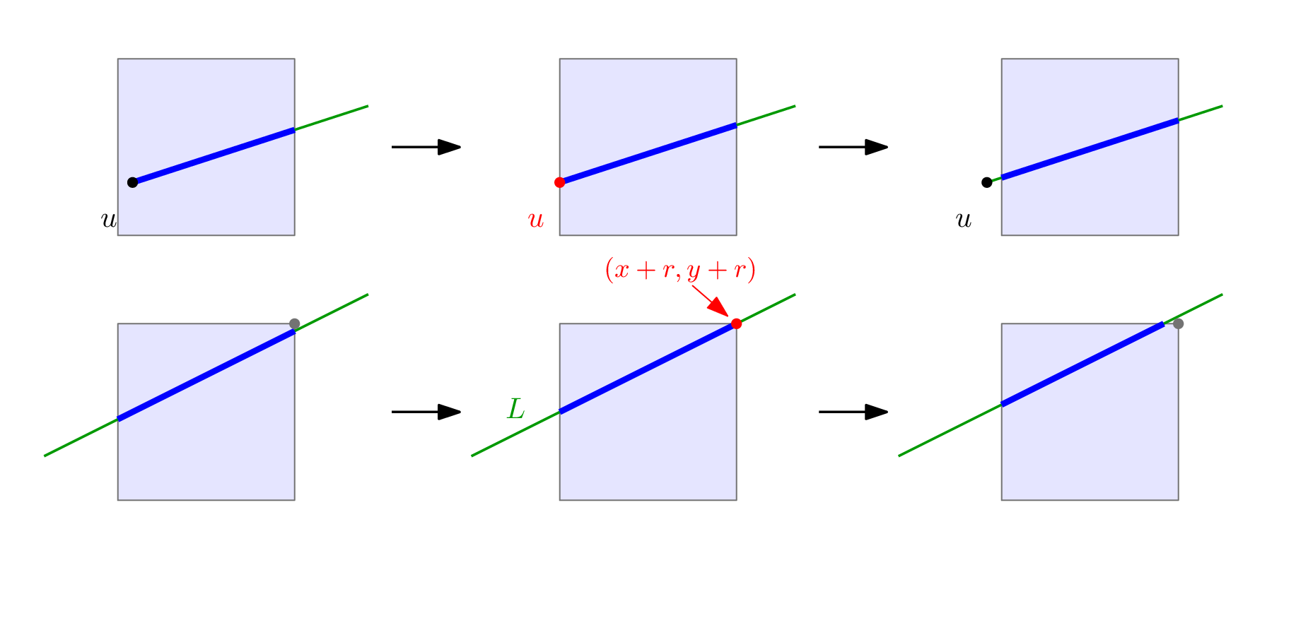
Figure 6.1: The clipping events in [Lemma 6.2](#x1-390012). Top row: endpoint $`u`$ crosses a square side ($`x-r=u_x`$). Bottom row: a square corner crosses the segment’s supporting line $`L`$ (green). Arrows show progression as the square moves right; blue highlights the clipped segment.

Let $`B=[x_{\min },x_{\max }]\times [y_{\min },y_{\max }]`$ be the input’s bounding rectangle, and let $`R`$ be half its larger side length. For every subset $`\mathcal{U}`$, the radius-$`R`$ square enclosing $`B`$ has congestion $`\left\|\mathcal{U}\right\|/R`$, at least that of any square of larger radius. Projecting a center into $`B`$ cannot increase its coordinatewise distance to any input point, so it cannot decrease clipped length. We may therefore clip the arrangement to the box $`B\times [0,R]`$. Including its six boundary planes gives at most $`12k+6`$ planes in total.

Within the relative interior of any face $`F`$ of this three-dimensional arrangement in $`r>0`$, the clipping pattern is fixed. Each clipped endpoint is either an original segment endpoint or the intersection of the segment with a fixed square side. Its position along the segment is therefore affine in $`(x,y,r)`$, and so is the clipped length. Consequently, for every subset $`\mathcal{U}`$, its total clipped length on $`F`$ is an affine function $`W_F(x,y,r)`$, and its congestion is <a id="x1-39009r3"></a>

```math
{\mathit{c}}_{\mathcal{U}}^{}\left({\Bigl .{\square}\left({\bigl .(x,y), r}\right)}\right) =\frac {W_F(x,y,r)}{r}. \tag{6.3}
```

This holds also on lower-dimensional faces, including those where a horizontal or vertical segment lies on a square side.

Extend $`W_F`$ affinely to the closure of $`F`$. Fixing $`r=\rho >0`$, maximizing congestion is equivalent to maximizing $`W_F`$ on the bounded slice $`\overline F\cap \{r=\rho \}`$. This affine function attains its maximum at a vertex of the slice. If this point is not already a vertex of $`\overline F`$, it lies on an edge transverse to the slice. Along this edge, $`x`$ and $`y`$ are affine functions of $`r`$, so the congestion has the form

```math
\frac {W_F(x(r),y(r),r)}{r}=\lambda _0+\frac {\lambda _1}{r}.
```

This is monotone or constant, so its maximum is at an endpoint. If an endpoint has $`r=0`$, then $`\lambda _1\leq 0`$, as otherwise $`W_F/r`$ would be unbounded on $`F`$ near this endpoint. The function is then nondecreasing in $`r`$, so the positive-radius endpoint is at least as good. At a boundary vertex the actual clipped length is at least its limit from $`F`$, because the square is closed. Thus some positive-radius vertex has congestion at least that of the original square.

Let $`\mathcal{V}`$ contain the squares of all positive-radius vertices of the clipped arrangement, together with one arbitrary square to cover the zero-congestion case. The arrangement depends only on the full input, so this family works for every subset simultaneously. It has at most $`\binom {12k+6}{3}+1\leq f(k)`$ members. Enumerating all triples of planes with independent normals produces all vertices, including those of degenerate arrangements. Evaluating the $`k`$ clipped lengths at every candidate gives the exact maximum in $`O((k+1)^4)`$ time. Empty input returns zero.

We use [Lemma 6.2](#x1-390012) in two ways. In the analysis of the sampling, in the next subsection, we apply it to the whole input $`{\mathcal{S}}`$ (so $`k=n`$). The resulting family $`\mathcal{V}`$ is determined by $`{\mathcal{S}}`$, and thus is fixed before any sampling takes place. This family is never constructed, as only its existence and its size are used. In the algorithm, we apply the lemma to the list of long segments of a cell, which has at most $`H_0`$ segments, where $`H_0=O_{{\varepsilon},q}(\log n)`$ is the cap set in [Section 6.5](#a-simple-stopping-rule), and there we do enumerate the vertices of its arrangement and compute the congestion of the list exactly.

<a id="x1-400006.3"></a><a id="sampling-at-geometrically-decreasing-rates"></a>

### 6.3  Sampling at geometrically decreasing rates

Assume that $`{\mathit{c}}\left({{\mathcal{S}}}\right)>0`$ (recall that the empty input is handled separately). Let $`0 < {\xi}\leq 1/20`$ be an accuracy parameter, and let $`0<\varphi<1`$ be the allowed failure probability. Define <a id="x1-40001r4"></a>

```math
\begin {split} J=\left\lceil {\log _2(n+2)} \right\rceil,\quad h=\log \bigl (2f(n)\tfrac { J+1}{\varphi} \bigr ), \quad \text {and}\quad T=\tfrac {24h}{{\xi}^2}. \end {split} \tag{6.4}
```

where $`f(n)=n^{O(1)}`$, see [Eq. (6.2)](#x1-39003r2).

The threshold $`T`$ depends only on $`n`$, $`{\xi}`$ and $`\varphi`$. The algorithm of [Section 6.5](#a-simple-stopping-rule) uses $`T`$ as the threshold of its stopping rule. For $`j=0,\ldots ,J`$, let $`{R}_j\subseteq {\mathcal{S}}`$ be a random sample that includes each segment of $`{\mathcal{S}}`$ independently with probability $`2^{-j}`$. The samples of different rounds are independent, and the algorithm computes a sample only when its round is reached.

<a id="lemma63"></a>

**Lemma 6.3.** <a id="x1-40003"></a><a id="x1-400023"></a>*With probability at least* $`1-\varphi`$*, we have, simultaneously for all* $`j`$*, that* <a id="x1-40004r5"></a>

```math
|{\mathit{c}}\left({{R}_j}\right)-2^{-j}{\mathit{c}}\left({{\mathcal{S}}}\right)|\leq {\xi}\max \{2^{-j}{\mathit{c}}\left({{\mathcal{S}}}\right),T\}. \tag{6.5}
```

<a id="proof12"></a>

*Proof:* <a id="x1-40006"></a>For a fixed round $`j\in \{0,\ldots ,J\}`$ and square $`{\square}\in \mathcal{V}`$ from [Lemma 6.2](#x1-390012), set $`X_j=\sum _{{s}\in {\mathcal{S}}}(I_{{s}}-2^{-j}){\mathit{c}}_{{s}}^{}\left({{\square}}\right)`$, where $`I_{{s}}`$ is the sampling indicator of $`{s}`$. Let $`p = \mathop{\mathbb{E}}\!\left[ {I_{s}} \right] = 1/2^j`$. We have $`{\mathbb{V}}\left[ I_{s}-p \right] = p ( 1-p) \leq p`$. Then, by the independence of these indicator variables, we have

```math
\begin{align*} {\mathbb{V}}\left[ X_j \right] &=\sum _{{s}\in {\mathcal{S}}}{\mathbb{V}}\left[ (I_{{s}}-2^{-j}){\mathit{c}}_{{s}}^{}\left({{\square}}\right) \right] \leq \sum _{{s}\in {\mathcal{S}}} {\mathit{c}}_{{s}}^{}\left({{\square}}\right)^2 {\mathbb{V}}\left[ I_{{s}} \right] \\&\leq p\sum _{{s}\in {\mathcal{S}}} {\mathit{c}}_{{s}}^{}\left({{\square}}\right)^2 \leq 3\cdot 2^{-j}\sum _{{s}\in {\mathcal{S}}}{\mathit{c}}_{{s}}^{}\left({{\square}}\right) \leq 3\cdot 2^{-j}{\mathit{c}}\left({{\mathcal{S}}}\right), \end{align*}
```

as $`{\mathit{c}}_{{s}}^{}\left({{\square}}\right)\leq \sqrt {8} \leq 3`$. Furthermore, $`|(I_{{s}}-2^{-j}){\mathit{c}}_{{s}}^{}\left({{\square}}\right)|\leq 3`$. Put $`V_j=\max \{2^{-j}{\mathit{c}}\left({{\mathcal{S}}}\right),T\}`$. [Bernstein’s inequality](#x1-490011), with $`T={24h}/{{\xi}^2}`$, gives

```math
\begin{align*} \mathop{\mathbb{P}\!\left[ {|X_j|>{\xi}V_j} \right]} &\leq 2\exp \left (-\frac {{\xi}^2V_j^2} {6\cdot 2^{-j}{\mathit{c}}\left({{\mathcal{S}}}\right)+2{\xi}V_j}\right )\\ &\leq 2\exp \left (-\frac {{\xi}^2T}{6+2}\right ) \leq 2\exp (-3h). \end{align*}
```

Union bound over at most $`f(n)(J+1)`$ choices of square and round gives the asserted probability. Both $`{\mathit{c}}\left({{\mathcal{S}}}\right)`$ and $`{\mathit{c}}\left({{R}_j}\right)`$ are maxima over the same family $`\mathcal{V}`$, so the deviation bound at those squares implies [Eq. (6.5)](#x1-40004r5).

We do not need a preliminary estimate of $`{\mathit{c}}\left({{\mathcal{S}}}\right)`$ to choose these rates or the threshold $`T`$. The stopping rule in [Section 6.5](#a-simple-stopping-rule) will certify that the accepted sample is sufficiently dense.

<a id="x1-410006.4"></a><a id="evaluation-with-bounded-conflict-lists"></a>

### 6.4  Evaluation with bounded conflict lists

We now describe the **evaluator**, the procedure that the final algorithm runs on each sample. Since it is applied to samples of the input rather than to the input itself, in this subsection the input is a multiset $`{\mathcal{S}}`$ of $`m`$ segments. Let $`P`$ be the set of distinct endpoints of the segments of $`{\mathcal{S}}`$, and fix an accuracy parameter $`0<{\xi}\leq 1/10`$. The evaluator also receives a failure probability $`0<\varphi<1`$, and a cap $`H_0\geq 1`$ on the size of the long lists it is willing to handle. The cap bounds the running time, and it is not an a priori bound on $`{\mathit{c}}\left({{\mathcal{S}}}\right)`$. If some long list has more than $`H_0`$ segments, the evaluator reports an overflow, which by [Observation 6.1](#x1-370011) certifies that $`{\mathit{c}}\left({{\mathcal{S}}}\right)>H_0/2`$. The evaluator first constructs a family $`{\Xi}`$ of $`O_{\xi}(m)`$ candidate squares, then builds the tight containment of $`{\Xi}`$, and finally computes two values for every retained cell, as described next.

<a id="x1-420006.4.1"></a><a id="the-candidate-squares"></a>

#### 6.4.1  The candidate squares

In the construction of the candidate squares, and in its analysis, distances and diameters are measured in the $`L_\infty`$ norm. Set $`\eta ={\xi}^2/100`$, and build a WSPD of $`P`$ with separation parameter $`\eta`$. That is, a set of $`O(m\eta ^{-2})`$ pairs $`(P_1,P_2)`$ of subsets of $`P`$, such that

```math
\max \{\mathrm{diam}\left({P_1}\right), \mathrm{diam}\left({P_2}\right)\} \leq \eta \operatorname {dist}_\infty (P_1,P_2)
```

for each pair $`(P_1,P_2)`$, and such that every two distinct points of $`P`$ are covered by some pair. Each pair $`(P_1,P_2)`$ comes with representatives $`a\in P_1`$ and $`a'\in P_2`$, and we denote $`d=\left\|a - a' \right\|_\infty >0`$. The pair contributes squares to $`{\Xi}`$ at the scales

```math
t_\ell =\frac {(1+{\xi})^\ell }{64},\qquad 0\leq \ell \leq J_{\mathrm {geo}},\qquad J_{\mathrm {geo}}=\left\lceil {\log _{1+{\xi}}(128/{\xi})} \right\rceil.
```

Specifically, for each scale $`t_\ell`$, let $`R=t_\ell d`$, and add to $`{\Xi}`$ the grid of squares around $`a`$ <a id="x1-42001r6"></a>

```math
{\square}\left({a+{\xi}R(i,j), (1+{\xi})R}\right), \qquad i,j\in \mathbb Z,\quad |i|,|j|\leq \left\lceil {2/{\xi}} \right\rceil, \tag{6.6}
```

and the corresponding grid of squares around $`a'`$. The family $`{\Xi}`$ is the set of all the squares added in this way, over all pairs and all scales. It has $`O(m{\xi}^{-7}\log (1/{\xi}))`$ squares.

<a id="lemma64ordinary-scales"></a>

**Lemma 6.4 (Ordinary scales).** <a id="x1-42003"></a><a id="x1-420024"></a>*Suppose* $`{\square}={\square}\left({{p}, r}\right)`$ *contains an endpoint* $`v`$ *and there is an endpoint* $`w`$ *with* <a id="x1-42004r7"></a>

```math
{\xi}r\leq \left\|v - w \right\|_\infty \leq 32r. \tag{6.7}
```

*Then some square of* $`{\Xi}`$ *contains* $`{\square}`$ *and has radius at most* $`(1+{\xi})^2r`$*.*

<a id="proof13"></a>

*Proof:* <a id="x1-42006"></a>Choose the WSPD pair covering $`v,w`$, and orient it so that $`v`$ belongs to the cluster represented by $`a`$. Put $`d_0=\left\|v - w \right\|_\infty`$. Separation gives

```math
|d-d_0|\leq 2\eta d_0,\qquad \left\|a - v \right\|_\infty \leq \eta d_0\leq 32\eta r\leq {\xi}r.
```

It follows that $`r/d\in [1/64,2/{\xi}]`$. Some chosen scale $`R`$ therefore satisfies $`r\leq R\leq (1+{\xi})r`$. Furthermore, $`\left\|{p} - a \right\|_\infty \leq (1+{\xi})r<2R`$. A grid center in [Eq. (6.6)](#x1-42001r6) lies within $`{\xi}R`$ of $`{p}`$, so its square of radius $`(1+{\xi})R`$ contains $`{\square}`$. Its radius is at most $`(1+{\xi})^2r`$.

<a id="x1-430006.4.2"></a><a id="the-same-squares-handle-isolated-endpoint-clusters"></a>

#### 6.4.2  The same squares handle isolated endpoint clusters

The following lemma handles squares for which [Lemma 6.4](#x1-420024) does not apply. In this case the endpoints near $`{\square}`$ form a tiny cluster, and the lemma shows that a square $`{\square}'\in {\Xi}`$ around this cluster has the following property. For any cell $`{C}`$ that tightly contains $`{\square}'`$ (as some retained cell of the tight containment does), the congestion of the long list of $`{C}`$, optimized over all squares, almost recovers the congestion of $`{\square}`$.

<a id="lemma65isolated-scales"></a>

**Lemma 6.5 (Isolated scales).** <a id="x1-43002"></a><a id="x1-430015"></a>*Let* $`{\square}={\square}\left({{p}, r}\right)`$ *contain an endpoint* $`v`$*, and suppose that* [Eq. (6.7)](#x1-42004r7) *fails for every endpoint* $`w`$*. Then one of the following holds:*

- **(I)** $`{\mathit{c}}_{{\mathcal{S}}}^{}\left({{\square}}\right)\leq 2{\xi}{\mathit{c}}\left({{\mathcal{S}}}\right)`$*, or*
- **(II)** *there is a square* $`{\square}'\in {\Xi}`$ *such that every square* $`{C}`$ *with* $`{\square}'\subseteq {C}`$ *and* $`{\mathsf{r}}\left({{C}}\right)\leq (1+{\xi}){\mathsf{r}}\left({{\square}'}\right)`$ *satisfies* <a id="x1-43005r8"></a>


  ```math
  {\mathit{c}}\left({{\mathcal{S}}_{\geq 1}\left({{C}}\right)}\right)\geq {\mathit{c}}_{{\mathcal{S}}}^{}\left({{\square}}\right)-2{\xi}{\mathit{c}}\left({{\mathcal{S}}}\right). \tag{6.8}
  ```



<a id="proof14"></a>

*Proof:* <a id="x1-43007"></a>The endpoints near $`v`$ form a tiny cluster $`U`$ surrounded by an empty annulus. A segment meeting $`{\square}`$ either has both endpoints in $`U`$, and then it is so short that it contributes little to the congestion of $`{\square}`$, or it has an endpoint outside the annulus, and then it is long for a suitable candidate square around the cluster. Formally, let $`U=P\cap {\square}\left({v, {\xi}r}\right)`$. Since [Eq. (6.7)](#x1-42004r7) fails for every endpoint $`w`$, every endpoint either lies in $`U`$, at distance less than $`{\xi}r`$ from $`v`$, or has distance greater than $`32r`$ from $`v`$. A segment with both endpoints in $`U`$ lies in $`{\square}\left({v, {\xi}r}\right)`$, so the total length of all such segments is at most $`{\xi}r{\mathit{c}}\left({{\mathcal{S}}}\right)`$, and their contribution to $`{\mathit{c}}_{{\mathcal{S}}}^{}\left({{\square}}\right)`$ is at most $`{\xi}{\mathit{c}}\left({{\mathcal{S}}}\right)`$. If $`U=P`$, every segment is of this kind, which gives the first alternative.

Suppose that $`U\neq P`$. Choose the nearest endpoint $`w\notin U`$ to $`v`$ in $`L_\infty`$, and put $`d_0=\left\|v - w \right\|_\infty >32r`$. Take the WSPD pair covering $`v,w`$, with representative $`a`$ on $`v`$’s side and representative distance $`d`$. Separation gives

```math
|d-d_0|\leq 2\eta d_0,\qquad \left\|a - v \right\|_\infty \leq \eta d_0<d_0.
```

By the choice of $`w`$, the last inequality forces $`a\in U`$, so $`\left\|a - v \right\|_\infty <{\xi}r`$.

The scales include some $`R`$ with $`d/8\leq R\leq (1+{\xi})d/8`$. Choose the candidate in [Eq. (6.6)](#x1-42001r6) centered exactly at $`a`$, with radius $`r'=(1+{\xi})R`$. Since $`{\xi}\leq 1/10`$, <a id="x1-43008r9"></a>

```math
d/8\leq r'\leq d/6,\qquad r'\geq (1-2\eta )d_0/8>(2+{\xi})r. \tag{6.9}
```

As $`v\in {\square}`$, we have $`\left\|{p} - a \right\|_\infty \leq (1+{\xi})r`$, so the square $`{\square}`$ lies in the interior of $`{\square}\left({a, r'}\right)={\square}'`$. Every outside endpoint $`z\notin U`$ satisfies

```math
\left\|z - a \right\|_\infty \geq d_0-{\xi}r > (1-{\xi}/32)d_0\geq d/2\geq 3r'.
```

Thus a segment meeting $`{\square}`$ and having an endpoint outside $`U`$ has length at least $`2r'`$, and it belongs to $`{\mathcal{S}}_{\geq 1}\left({{C}}\right)`$ for any $`{C}`$ as in the statement, since it meets the interior of $`{C}\supseteq {\square}'`$ and $`{\mathsf{r}}\left({{C}}\right)\leq (1+{\xi})r'<2r'`$.

Hence every segment meeting $`{\square}`$, except those with both endpoints in $`U`$, belongs to $`{\mathcal{S}}_{\geq 1}\left({{C}}\right)`$. By the first paragraph,

```math
{\mathit{c}}\left({{\mathcal{S}}_{\geq 1}\left({{C}}\right)}\right) \geq {\mathit{c}}_{{\mathcal{S}}_{\geq 1}\left({{C}}\right)}^{}\left({{\square}}\right) \geq {\mathit{c}}_{{\mathcal{S}}}^{}\left({{\square}}\right)-{\xi}{\mathit{c}}\left({{\mathcal{S}}}\right),
```

which is stronger than [Eq. (6.8)](#x1-43005r8).

Note that the cluster $`U`$ and the endpoint $`w`$ are used only in the analysis. The algorithm does not need to identify isolated clusters, as the family $`{\Xi}`$ already contains the square $`{\square}'`$.

<a id="x1-440006.4.3"></a><a id="evaluation-and-approximation-guarantee"></a>

#### 6.4.3  Evaluation and approximation guarantee

The evaluator builds the tight containment of $`{\Xi}`$ with parameters $`\delta ={\xi}`$ and $`\varphi`$, and registers the segments of $`{\mathcal{S}}`$ in each tree with the long threshold $`{\alpha}=1`$. It then computes the long list $`{\mathcal{S}}_{\geq 1}\left({{C}}\right)`$ of every retained cell $`{C}`$ by the traversal of [Lemma 4.2](#x1-230012) with threshold $`H_0`$, and reports an overflow if some list exceeds $`H_0`$. Otherwise, for every retained cell $`{C}`$, it computes the following two values.

- **(I)** The exact congestion $`{\mathit{c}}_{{\mathcal{S}}}^{}\left({{C}}\right)`$ of the cell. This is its exact short congestion plus the lengths of the segments of $`{\mathcal{S}}_{\geq 1}\left({{C}}\right)`$ clipped to $`{C}`$, divided by the radius of $`{C}`$.
- **(II)** The congestion $`{\mathit{c}}\left({{\mathcal{S}}_{\geq 1}\left({{C}}\right)}\right)`$ of the segments of its long list, computed exactly using [Lemma 6.2](#x1-390012). Here the segments are not clipped to $`{C}`$, and the maximum is over all squares. In particular, the square realizing this maximum may be far smaller than $`{C}`$, or have a different center. Its location is not constrained by the tree.

The two cases are illustrated in [Figure 6.2](#a-c-evaluate-c-s-c-b-evaluate-c-s-1-c-over-all-squares-here-s-is-the-depicted-segment-set-and-the-red-dot-represents-the-cluster-u-containing-v-arrows-continue-to-endpoints-outside-u-more-than-32-r-from-v). The evaluator returns the largest of all these values, denoted by $`B`$. Every cell is a square and every long list is a subset of $`{\mathcal{S}}`$, so both kinds of values are at most $`{\mathit{c}}\left({{\mathcal{S}}}\right)`$, and $`B\leq {\mathit{c}}\left({{\mathcal{S}}}\right)`$.

<a id="a-c-evaluate-c-s-c-b-evaluate-c-s-1-c-over-all-squares-here-s-is-the-depicted-segment-set-and-the-red-dot-represents-the-cluster-u-containing-v-arrows-continue-to-endpoints-outside-u-more-than-32-r-from-v"></a>

![evaluator cases-](assets/evaluator_cases-.png) <a id="x1-44003r2"></a>

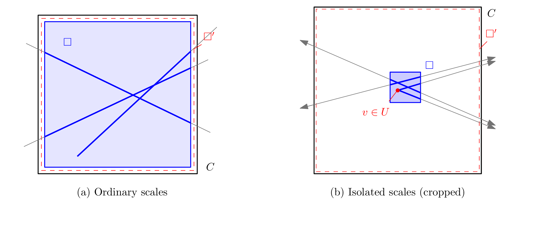
Figure 6.2: (a) $`{\square}\subseteq {\square}'\subseteq {C}`$; evaluate $`{\mathit{c}}_{{\mathcal{S}}}^{}\left({{C}}\right)`$. (b) Evaluate $`{\mathit{c}}\left({{\mathcal{S}}_{\geq 1}\left({{C}}\right)}\right)`$ over all squares. Here $`{\mathcal{S}}`$ is the depicted segment set, and the red dot represents the cluster $`U`$ containing $`v`$. Arrows continue to endpoints outside $`U`$, more than $`32{\mathsf{r}}\left({{\square}}\right)`$ from $`v`$.

<a id="lemma66boundedlist-evaluator"></a>

**Lemma 6.6 (Bounded-list evaluator).** <a id="x1-44005"></a><a id="x1-440046"></a>*Given a multiset* $`{\mathcal{S}}`$ *of* $`m`$ *segments and a cap* $`H_0\geq 1`$*, the evaluator either reports an overflow, which certifies that* $`{\mathit{c}}\left({{\mathcal{S}}}\right)>H_0/2`$*, or returns a value* $`B\leq {\mathit{c}}\left({{\mathcal{S}}}\right)`$*. With probability at least* $`1-\varphi`$*, a returned value also satisfies*

```math
B\geq (1-3{\xi}){\mathit{c}}\left({{\mathcal{S}}}\right).
```

*The running time is*

```math
O_{\xi}\bigl (m\log ^2((m+2)/\varphi) +m(H_0+1)^4\log ((m+2)/\varphi)\bigr ).
```

*For an empty input the evaluator returns zero immediately.*

<a id="proof15"></a>

*Proof:* <a id="x1-44007"></a>The lower bound on $`B`$ is the heart of the proof. We take a square $`{\square}`$ with congestion close to $`{\mathit{c}}\left({{\mathcal{S}}}\right)`$, argue that we can assume that it contains an endpoint, and then apply [Lemma 6.4](#x1-420024) or [Lemma 6.5](#x1-430015), depending on whether or not $`{\square}`$ has an endpoint $`w`$ satisfying [Eq. (6.7)](#x1-42004r7), to show that one of the values computed by the evaluator is almost $`{\mathit{c}}_{{\mathcal{S}}}^{}\left({{\square}}\right)`$.

Condition on the event that every square of $`{\Xi}`$ is contained in a retained cell of radius at most $`(1+{\xi})`$ times its own, and suppose that no list overflows. Consider a square $`{\square}={\square}\left({{p}, \rho }\right)`$ whose congestion is arbitrarily close to $`{\mathit{c}}\left({{\mathcal{S}}}\right)`$. If $`{\square}`$ contains no endpoint, enlarge it concentrically until its boundary meets an endpoint. We claim that the congestion does not decrease. Indeed, while no endpoint is inside, every contributing segment meets the square in the full chord of its supporting line $`L`$, and scaling by $`1/\rho`$ about $`{p}`$ shows that $`\left\|L\cap {\square}\left({{p}, \rho }\right)\right\|/\rho`$ is the chord length of the fixed square $`{\square}\left({{p}, 1}\right)`$ along a line parallel to $`L`$ at Euclidean distance $`\operatorname {dist}({p},L)/\rho`$ from $`{p}`$. This distance does not increase as $`\rho`$ grows, and the chord lengths of a centrally symmetric convex region along parallel lines form an even concave function of the offset, so they do not decrease as the offset moves toward zero. Segments that start meeting the square during the enlargement only add length. Thus we may assume that $`{\square}={\square}\left({{p}, r}\right)`$ contains an endpoint $`v`$.

If there is an endpoint $`w`$ satisfying [Eq. (6.7)](#x1-42004r7), then by [Lemma 6.4](#x1-420024) some square of $`{\Xi}`$ contains $`{\square}`$ and has radius at most $`(1+{\xi})^2r`$, and by tight containment some retained cell $`{C}`$ contains this square and has radius at most $`(1+{\xi})^3r`$. Since $`{\square}\subseteq {C}`$, the exact congestion of $`{C}`$, which is the first value computed by the evaluator, is at least

```math
\frac {{\mathit{c}}_{{\mathcal{S}}}^{}\left({{\square}}\right)}{(1+{\xi})^3} \geq (1-3{\xi}){\mathit{c}}_{{\mathcal{S}}}^{}\left({{\square}}\right).
```

Otherwise, [Eq. (6.7)](#x1-42004r7) fails for every endpoint $`w`$, and [Lemma 6.5](#x1-430015) applies. Its first alternative, $`{\mathit{c}}_{{\mathcal{S}}}^{}\left({{\square}}\right)\leq 2{\xi}{\mathit{c}}\left({{\mathcal{S}}}\right)`$, cannot hold once $`{\mathit{c}}_{{\mathcal{S}}}^{}\left({{\square}}\right)`$ is close enough to $`{\mathit{c}}\left({{\mathcal{S}}}\right)`$, which is positive for a nonempty input. So there is a square $`{\square}'\in {\Xi}`$ as in the second alternative, and by tight containment some retained cell $`{C}`$ contains $`{\square}'`$ and has radius at most $`(1+{\xi}){\mathsf{r}}\left({{\square}'}\right)`$. By [Eq. (6.8)](#x1-43005r8), the second value computed by the evaluator for $`{C}`$, namely $`{\mathit{c}}\left({{\mathcal{S}}_{\geq 1}\left({{C}}\right)}\right)`$, is at least $`{\mathit{c}}_{{\mathcal{S}}}^{}\left({{\square}}\right)-2{\xi}{\mathit{c}}\left({{\mathcal{S}}}\right)`$. In both cases, letting $`{\mathit{c}}_{{\mathcal{S}}}^{}\left({{\square}}\right)`$ tend to $`{\mathit{c}}\left({{\mathcal{S}}}\right)`$ proves $`B\geq (1-3{\xi}){\mathit{c}}\left({{\mathcal{S}}}\right)`$. The upper bound $`B\leq {\mathit{c}}\left({{\mathcal{S}}}\right)`$ holds unconditionally, as every cell is a square and every list is a subset of the input.

As for the running time, the traversal stops on the first list exceeding $`H_0`$, and such a list certifies $`{\mathit{c}}\left({{\mathcal{S}}}\right)>H_0/2`$ by [Observation 6.1](#x1-370011). Otherwise, there are $`O_{\xi}(\log ((m+2)/\varphi))`$ trees with $`O_{\xi}(m)`$ retained cells each, and the exact optimization of [Lemma 6.2](#x1-390012) costs $`O((H_0+1)^4)`$ per cell, which gives the second term of the bound. The construction of the trees, the registration of the segments, the computation of the short congestions, and the enumeration of the long lists all fit in the stated bound.

<a id="x1-450006.5"></a><a id="a-simple-stopping-rule"></a>

### 6.5  A simple stopping rule

We now put everything together, reusing the sampling and exponential-search framework of [Section 4](#approximating-the-maximum-load-of-the-long-segments-in-a-quadtree), where we now test the congestion of the sample instead of its maximum long list size. The algorithm runs the evaluator on samples of decreasing density. A round is rejected if its sample is too dense, that is, if a long list overflows or the returned value exceeds the threshold $`T`$.

<a id="algorithm61sampling-for-square-congestion"></a>

Algorithm 6.1 (Sampling for square congestion). <a id="x1-45002"></a><a id="x1-450011"></a>Given $`n`$ segments $`{\mathcal{S}}`$, an approximation parameter $`{\varepsilon}>0`$, and a confidence parameter $`q>0`$:

- **(A)** Set $`{\xi}=\min \{{\varepsilon},1\}/20`$ and $`\varphi=\tfrac 12(n+2)^{-q}`$. Compute $`J`$ and $`T`$ from [Eq. (6.4)](#x1-40001r4), and set $`H_0=\left\lceil {2T} \right\rceil`$.
- **(B)** For $`j=0,1,\ldots ,J`$, in this order:
  - **(i)** Form $`{R}_j`$ by including each segment of $`{\mathcal{S}}`$ independently with probability $`2^{-j}`$.
  - **(ii)** Run the evaluator of [Lemma 6.6](#x1-440046) on $`{R}_j`$ with cap $`H_0`$ and failure probability $`\varphi/(J+1)`$.
  - **(iii)** If it reports an overflow or returns $`B_j>T`$, continue with the next round. Otherwise, stop and return <a id="x1-45008r10"></a>


    ```math
    A=\frac {1-{\xi}}{1+{\xi}}\,2^jB_j. \tag{6.10}
    ```


- **(C)** Return zero if all rounds were rejected.

The final return of zero only guarantees that the algorithm terminates within the stated running time. We show below that, when the algorithm succeeds, some round is accepted, so the fallback is never used.

<a id="theorem67"></a>

**Theorem 6.7.** <a id="x1-45011"></a><a id="x1-450107"></a>*Let* $`{\mathcal{S}}`$ *be a set of* $`n`$ *segments in the plane, and let* $`{\varepsilon}>0`$ *and* $`q>0`$ *be fixed. The above algorithm returns a number* $`A`$ *such that*

```math
A\leq {\mathit{c}}\left({{\mathcal{S}}}\right)\leq (1+{\varepsilon})A
```

*with probability at least* $`1-(n+2)^{-q}`$*. Its running time is* $`O_{{\varepsilon},q}(n\log ^6(n+2))`$ *in the worst case and* $`O_{{\varepsilon},q}(n\log ^5(n+2))`$ *in expectation, in the same model of computation as in the preceding sections. In particular, the number of candidate scales, and the running time, do not depend on the spread of the coordinates of the input.*

<a id="proof16"></a>

*Proof:* <a id="x1-45013"></a>The proof has three parts. We first show that some round is accepted. We then show that the sample of the accepted round is dense enough for [Eq. (6.5)](#x1-40004r5) to give a relative error, which yields the approximation guarantee. Finally, we bound the running time.

Condition on the event of [Lemma 6.3](#x1-400023), for all rounds simultaneously, and on the success of the tight containment in every evaluator that is executed. By the union bound, the total failure probability is at most $`2\varphi=(n+2)^{-q}`$.

Since $`{\mathit{c}}\left({{\mathcal{S}}}\right)\leq 3n`$, by [Eq. (6.1)](#x1-34001r1), and $`2^{-J}\leq 1/(n+2)`$, we have $`2^{-J}{\mathit{c}}\left({{\mathcal{S}}}\right)\leq 3`$. The definition of $`T`$ gives $`3\leq (1-{\xi})T`$, and therefore, by [Eq. (6.5)](#x1-40004r5),

```math
{\mathit{c}}\left({{R}_J}\right)\leq 2^{-J}{\mathit{c}}\left({{\mathcal{S}}}\right)+{\xi}T\leq T.
```

By [Observation 6.1](#x1-370011), every long list in round $`J`$ has size at most $`2T\leq H_0`$, so no list overflows, and the returned value satisfies $`B_J\leq {\mathit{c}}\left({{R}_J}\right)\leq T`$. Consequently, round $`J`$ is accepted if it is reached, and in any case some round is accepted.

Let $`j`$ be the index of the accepted round, and suppose first that $`j>0`$. Round $`j-1`$ was rejected, and this certifies that $`{\mathit{c}}\left({{R}_{j-1}}\right)>T`$. Indeed, either a list overflowed, and then $`{\mathit{c}}\left({{R}_{j-1}}\right)>H_0/2\geq T`$ by [Lemma 6.6](#x1-440046), or the returned value satisfied $`B_{j-1}>T`$, and $`{\mathit{c}}\left({{R}_{j-1}}\right)\geq B_{j-1}`$. We claim that

```math
2^{1-j}{\mathit{c}}\left({{\mathcal{S}}}\right)>(1-{\xi})T.
```

Indeed, if $`2^{1-j}{\mathit{c}}\left({{\mathcal{S}}}\right)\leq (1-{\xi})T`$, then [Eq. (6.5)](#x1-40004r5) would give $`{\mathit{c}}\left({{R}_{j-1}}\right)\leq 2^{1-j}{\mathit{c}}\left({{\mathcal{S}}}\right)+{\xi}T\leq T`$, a contradiction. Thus, the accepted round satisfies $`T<2^{1-j}{\mathit{c}}\left({{\mathcal{S}}}\right)/(1-{\xi})`$, so the deviation permitted by [Eq. (6.5)](#x1-40004r5) is $`{\xi}\max \{2^{-j}{\mathit{c}}\left({{\mathcal{S}}}\right),T\} \leq \tfrac {2{\xi}}{1-{\xi}}2^{-j}{\mathit{c}}\left({{\mathcal{S}}}\right)`$, and <a id="x1-45014r11"></a>

```math
\frac {1-3{\xi}}{1-{\xi}}\,2^{-j}{\mathit{c}}\left({{\mathcal{S}}}\right) \leq {\mathit{c}}\left({{R}_j}\right)\leq \frac {1+{\xi}}{1-{\xi}}\,2^{-j}{\mathit{c}}\left({{\mathcal{S}}}\right). \tag{6.11}
```

If $`j=0`$, then $`{R}_0={\mathcal{S}}`$, so [Eq. (6.11)](#x1-45014r11) holds trivially. By [Lemma 6.6](#x1-440046), the evaluator gives $`(1-3{\xi}){\mathit{c}}\left({{R}_j}\right)\leq B_j\leq {\mathit{c}}\left({{R}_j}\right)`$. Multiplying through by $`2^j(1-{\xi})/(1+{\xi})`$, the returned value obeys

```math
A\leq {\mathit{c}}\left({{\mathcal{S}}}\right) \qquad \text {and}\qquad \frac {{\mathit{c}}\left({{\mathcal{S}}}\right)}{A}\leq \frac {1+{\xi}}{(1-3{\xi})^2}.
```

For $`0<{\xi}\leq 1/20`$,

```math
\frac {1+{\xi}}{(1-3{\xi})^2}-1 =\frac {7{\xi}-9{\xi}^2}{(1-3{\xi})^2} \leq 10{\xi}\leq {\varepsilon}.
```

This proves the approximation guarantee.

It remains to bound the running time. By [Eq. (6.4)](#x1-40001r4), $`h=O_q(\log (n+2))`$, so the cap is $`H_0=\left\lceil {2T} \right\rceil=O_{{\varepsilon},q}(\log (n+2))`$. By [Lemma 6.6](#x1-440046), the evaluator of round $`j`$ thus takes $`O_{{\varepsilon},q}(m_j\log ^5(n+2))`$ time, where $`m_j`$ is the size of its sample, plus the $`O(n)`$ time needed to draw the sample. There are $`O(\log (n+2))`$ rounds, which gives the claimed worst-case bound. For the expectation, conceptually draw all rounds, including those after stopping. Their expected total size is

```math
\sum _{j=0}^J\mathop{\mathbb{E}}\!\left[ {m_j} \right] =n\sum _{j=0}^J2^{-j}<2n.
```

Stopping only reduces the work, so the expected time is $`O_{{\varepsilon},q}(n\log ^5(n+2))`$.

<a id="x1-460007"></a><a id="conclusions"></a>

## 7  Conclusions

We provided a near-linear time algorithm that computes a constant factor approximation to the congestion of a polygonal curve (i.e., the minimum $`c`$ such that the curve is $`c`$-packed). We consider the result to be quite surprising, even though the constant is undesirably large (i.e., $`42`$). We then showed, in [Section 6](#a-1-approximation-in-nearlinear-time), using AI to develop this part, that the approximation factor can be improved to $`1+{\varepsilon}`$, for any fixed $`{\varepsilon}>0`$, while keeping the running time near-linear.

The constant factor algorithm of [Section 5](#approximating-the-maximum-congestion) works verbatim in any constant dimension – it has not used planarity in any way. The quality of approximation deteriorates with the dimension $`d`$, but it is still a constant when $`d`$ is a constant. The running time remains $`O(n \log ^3 n)`$. Extending the $`(1+{\varepsilon})`$-approximation of [Section 6](#a-1-approximation-in-nearlinear-time) to higher dimensions is left for future work. Another important property of our algorithms is that they do not require the input segments to form a curve.

The dependence on $`{\varepsilon}`$, and the number of logarithmic factors, in the running time of the algorithm of [Section 6](#a-1-approximation-in-nearlinear-time) are likely far from optimal. Improving them is an interesting problem for future research.

Nothing in our algorithm is a no-starter from a practical point of view. Performing an experimental study using this algorithm is an interesting direction for future research.

<a id="acknowledgements"></a> **<a id="x1-47000"></a>Acknowledgements.** Work on this paper started more than a decade ago in a collaboration between the first author and Anne Driemel. The authors thank the anonymous referees for their detailed and insightful comments that significantly improved this work.

<a id="x1-48000"></a>

### References

\[AH08\]
<a id="Xah-adrp-08"></a>B. Aronov and S. Har-Peled. On approximating the depth and related problems. *SIAM J. Comput.*, 38(3):899–921, 2008.

\[AKGM20\]
<a id="Xakgm-wqmse-20"></a>Sepideh Aghamolaei, Vahideh Keikha, Mohammad Ghodsi, and Ali Mohades. Windowing queries using Minkowski sum and their extension to mapreduce. *J. Supercomput.*, April 2020.

\[Alt09\]
<a id="Xa-cgcs"></a>Helmut Alt. *Efficient Algorithms: Essays Dedicated to Kurt Mehlhorn on the Occasion of His 60th Birthday*, chapter The Computational Geometry of Comparing Shapes, page 235–248. Springer-Verlag, 2009.

\[BHR<sup>+</sup>20\]
<a id="Xbhrrs-eeiso-20"></a>Paul Beame, Sariel Har-Peled, Sivaramakrishnan Natarajan Ramamoorthy, Cyrus Rashtchian, and Makrand Sinha. Edge estimation with independent set oracles. *ACM Trans. Algo.*, 16(4), September 2020.

\[Bri14\]
<a id="Xb-wwdtt-14"></a>K. Bringmann. Why walking the dog takes time: Frechet distance has no strongly subquadratic algorithms unless SETH fails. In *Proc. 55th Annu. IEEE Sympos. Found. Comput. Sci.* (FOCS), pages 661–670, 2014.

\[DHW12\]
<a id="Xdhw-afdrc-12"></a>A. Driemel, S. Har-Peled, and C. Wenk. Approximating the Fréchet distance for realistic curves in near linear time. *Disc. Comput. Geom.*, 48:94–127, 2012.

\[Eri95\]
<a id="Xe-rcsgp"></a>Jeff Erickson. On the relative complexities of some geometric problems. *Proc. 7th Canadian Conference on Computational Geometry*, page 85–90, 1995.

\[GSW20\]
<a id="Xgsw-appc-20"></a>Joachim Gudmundsson, Yuan Sha, and Sampson Wong. Approximating the packedness of polygonal curves. *CoRR*, abs/2009.07789, 2020. to appear in ISAAC 2020.

\[GvKS13\]
<a id="Xgks-alhctd-13"></a>Joachim Gudmundsson, Marc van Kreveld, and Frank Staals. Algorithms for hotspot computation on trajectory data. In *Proc. 21st ACM SIG. Int. Conf. Adv. Geo. Info. Sys. (SIGSPATIAL)*, SIGSPATIAL’13, page 134–143, New York, NY, USA, 2013. Association for Computing Machinery.

\[Har11\]
<a id="Xh-gaa-11"></a>S. Har-Peled. *Geometric Approximation Algorithms*, volume 173 of *Math. Surveys & Monographs*. Amer. Math. Soc., Boston, MA, USA, 2011.

\[Vig14\]
<a id="Xv-gosaf-14"></a>A. Vigneron. Geometric optimization and sums of algebraic functions. *ACM Trans. Algo.*, 10(1):4:1–4:20, 2014.

\[Wil15\]
<a id="Xw-hepbh-15"></a>Virginia Vassilevska Williams. Hardness of easy problems: Basing hardness on popular conjectures such as the strong exponential time hypothesis (invited talk). In Thore Husfeldt and Iyad A. Kanj, editors, *10th Int. Symp. Param. Exact Comput, IPEC*, volume 43 of *LIPIcs*, pages 17–29. Schloss Dagstuhl - Leibniz-Zentrum für Informatik, 2015.

<a id="x1-49000A"></a><a id="bernsteins-inequality"></a>

## A  Bernstein’s inequality

<a id="theorema1bernsteins-inequality"></a>

**Theorem A.1 (Bernstein’s inequality).** <a id="x1-49002"></a><a id="x1-490011"></a>*Let* $`X_1,\ldots ,X_m`$ *be independent real random variables with* $`\mathop{\mathbb{E}}\!\left[ {X_i} \right]=0`$ *and* $`|X_i|\leq L`$ *almost surely, where* $`L>0`$*. Set* $`X=\sum _{i=1}^m X_i`$ *and* $`\sigma ^2=\sum _{i=1}^m{\mathbb{V}}\left[ X_i \right]`$*. Then, for every* $`t>0`$*,*

```math
\mathop{\mathbb{P}\!\left[ {|X|\geq t} \right]} \leq 2\exp \left (-\frac {t^2}{2\sigma ^2+(2/3)Lt}\right ).
```

<a id="x2-18004x1"></a> <a id="fn1x0"></a><sup>1</sup>Spoiler alert! The butler did it, $`{\alpha}=20`$, and the hero dies in the end. The hero did try to expose $`{\alpha}`$, but it was too late for them.

<a id="x3-31006x2"></a> <a id="fn2x0"></a><sup>2</sup>So, confusingly, while the winning estimate might not be from the node with the largest conflict list, it comes from a node with a conflict list of size very close to it – if it was much smaller, it would not have been able to beat it.

<a id="x4-32002x5"></a> <a id="fn3x0"></a><sup>3</sup>Spoiler alert! The hero is still dead, and it turns out that for $`{\mathcal{T}}_1, \ldots , {\mathcal{T}}_m`$ the quadtrees of [Lemma 3.3](#x1-150083), $`\max _i {\mathcal{C}}^{}_{\!\hspace{0.6pt}\geq {\alpha}}({\mathcal{T}}_i)`$ is a good approximation to $`{\mathit{c}}\left({{\mathcal{S}}}\right)`$.