Batch Tree-Path Maxima and Minimum Spanning Tree Verification

Authoritative PDF · Markdown reading copy

Sariel Har-Peled∗

∗School of Computing and Data Science; University of Illinois; 201 N. Goodwin Avenue; Urbana, IL, 61801, USA; sariel@illinois.edu; http://sarielhp.org/. Work on this paper was partially supported by NSF AF award CCF-2317241.

Abstract

We describe a deterministic variant of the King–Hagerup framework for batch tree-path maxima and minimum spanning tree verification. Allowing unused candidates to remain eliminates set projection: the algorithm searches over demand depths and updates candidates by retaining a prefix and appending the incoming edge. A median lookup table supports ordinary binary search. The algorithm returns all requested path-maximum weights in deterministic linear time under the word-RAM model.

1 Introduction

Given a weighted tree and a batch of vertex pairs, the tree-path-maxima problem asks for the maximum edge weight on each corresponding tree path. Minimum spanning tree (MST) verification is an application: compare each non-tree, non-loop edge with the maximum weight on its path in the proposed tree. We describe a deterministic variant of an existing linear-time framework, with the aim of reducing the machinery needed for query processing.

Approach and relation to previous work. King [Kin97] reduces the problem to ancestor–descendant queries in a balanced hierarchy, using Borůvka’s construction and lowest common ancestor (LCA) preprocessing. Hagerup [Hag10] gives a deterministic linear-time algorithm for these queries, maintaining query-dependent sets of suffix maxima. His algorithm uses a set-projection operation and binary searches supported by a table of medians of bit masks. Zwick [Zwi09] presents the King–Hagerup algorithm with a direct invariant on the current answers, which is also the form of our correctness argument, and outlines table-based implementations of the required operations on word fragments. We retain the hierarchy and LCA reduction, but allow candidate sets to contain edges that represent no current query. This permits an update that keeps a prefix of the old candidates and appends the new edge, without set projection. Binary search runs on the demand depths, obtaining each old answer by a single successor lookup in the candidate mask. Searching the demands keeps the cost dependent on their number, even when unused candidates remain. We retain median-table lookup. The hierarchy height is at most \(\lfloor \log n\rfloor\), so a table for every possible demand mask has at most \(n\) entries. Removing the smallest and largest set bits gives a constant-time recurrence for filling each entry.

Scope and limitations. The result returns all requested path maxima exactly and retains Hagerup’s deterministic linear-time guarantee. The change is a local simplification of the update and its implementation within the existing framework. It gives no asymptotic improvement in time or space. The simplification concerns the query-processing stage: the hierarchy construction remains, and LCA preprocessing is used as a black box. Some of the shorter proof arguments can also be used to explain earlier algorithms. The comparison therefore concerns both the algorithm and its presentation, and establishes neither a practical speed advantage nor a ranking among all approaches. The theorem assumes distinct edge weights and the word-RAM operations specified below.

AI provenance. This work was carried out by AI assistants through OpenAI Codex under human direction. The assistants developed the algorithmic variant within the cited framework, drafted and revised the proofs, wrote implementations, and prepared this manuscript. Human input supplied the research questions, mathematical suggestions, and critical feedback that guided the work. This manuscript is presented as an AI-generated research draft.

Problem and output. Throughout, assume \(n>1\) and, for simplicity of exposition, that the input edge weights are pairwise distinct.

Definition 1.1. Let \(T=(V,E_T)\) be an undirected tree on \(n>1\) vertices, with pairwise distinct finite real edge weights \(w:E_T\to \mathbb {R}\). For distinct vertices \(u,v\), let \(P_T(u,v)\) denote their unique tree path and define its path maximum by

\[w_{T}^{}(u,v)=\max \left\{ \bigl .w(e) \;\middle\vert\; e\in P_T(u,v) \right\}.\]

A batch of path queries is an indexed list \(\mathcal{Q}=\bigl ((u_i,v_i)\bigr )_{i=1}^{s}\) of pairs with \(u_i\ne v_i\). Repeated pairs are allowed. The output is \(w_{T}^{}(u_i,v_i)\), for \(i=1,\ldots ,s\).

Problem 1.2. The input is a connected, undirected graph \(G=(V,E)\), with \(n>1\) vertices, \(m\) edges with pairwise distinct finite real weights, and a list of edges specifying a proposed tree \(T\). Parallel edges and loops are allowed. A spanning tree connects all vertices without cycles. It is a minimum spanning tree if its total edge weight is smallest among all spanning trees of \(G\).

The output first states whether \(T\) is a spanning tree. If it is, then for every non-loop edge \(e=uv\) the output contains \(w_{T}^{}(u,v)\) and its edge classification: \(w(e)<w_{T}^{}(u,v)\), \(w(e)=w_{T}^{}(u,v)\), or \(w(e)>w_{T}^{}(u,v)\). Equality holds exactly for tree edges; every other non-loop edge is lighter or heavier than its path maximum. The output also states whether \(T\) is minimum. An edge \(e\) with \(w(e)<w_{T}^{}(u,v)\) is a violating edge.

If \(T\) is not spanning, the algorithm reports it and exits.

Computational model and main result. The bounds use a word RAM with word length \(W=\Theta (\log (n+s))\) for batch queries and \(W=\Theta (\log (n+m))\) for MST verification. Array access, integer arithmetic on these words, Boolean operations, shifts, and finding the first or last set bit take constant time. Edge weights are atomic values that can be copied and compared in constant time. In particular, the algorithm does not sort them or use arithmetic on them. All logarithms are in base two.

Under this model, we answer all \(s\) path queries exactly in deterministic \(O(n+s)\) time and \(O(n+s)\) space, including lookup-table construction. This gives MST verification in deterministic \(O(n+m)\) time and \(O(n+m)\) space; see Theorem 6.1.

Sketch of algorithm. Four stages make the bound possible.

(A) Build a shallow weighted hierarchy whose leaves are the vertices of \(T\) and whose leaf-to-leaf path maxima agree with those of \(T\) (Section 3).

(B) Preprocess the hierarchy for lowest common ancestor queries. Split each queried path at its lowest common ancestor into two ancestor–leaf queries (Section 4).

(C) Collect the query depths by a bottom-up union (Section 5) and construct the median table (Section 2).

(D) Traverse downward, binary-searching each demand mask to update the candidates, and answer queries at the leaves. The logarithmic search costs sum to linear time over the hierarchy (Section 6).

2 Preliminaries

2.1 Small integer sets

For an integer \(k\geq 0\), write \([k]=\{1,\ldots ,k\}\), with \([0]=\varnothing\). A set \(S\subseteq \{0,\ldots ,b\}\), where \(b=O(\log n)\), is represented by its mask \(\mathop{\mathrm{mask}}(S)=\sum _{t\in S}2^t\), using \(O(1)\) words. We identify sets with their masks: \(\cup\) and \(\cap\) are implemented by bitwise OR and AND, respectively. Write \(\operatorname{Low}(t)=2^t-1\) for the mask of positions \(0,\ldots ,t-1\).

For a set \(S\) and a nonnegative integer \(q\), define its strict successor by

\[\mathop{\mathrm{succ}}(S,q)=\min \left\{ t\in S \;\middle\vert\; t>q \right\},\]

with value \(\bot\) if there is none. To compute it, shift the mask right by \(q+1\) bits, setting \(Y=S\mathbin{\gg}(q+1)\): return \(\bot\) if \(Y=0\), and otherwise return \(q+1+\mathop{\mathrm{\mathrm{lsb}}}(Y)\), where \(\mathop{\mathrm{\mathrm{lsb}}}\) is the zero-based index of the lowest set bit. An increasing scan repeatedly extracts the lowest set bit and clears it by \(Y\leftarrow Y-2^{\mathop{\mathrm{\mathrm{lsb}}}(Y)}\). These operations take constant time per lookup or scanned position.

2.2 Median lookup and binary search

For a nonempty ordered set \(D=\{q_0<\cdots <q_{k-1}\}\), its upper median is \(q_{\lfloor k/2\rfloor }\). A table of these medians makes each binary-search pivot available in constant time.

Lemma 2.1 (Median table). For an integer \(1\leq h\leq \lfloor \log n\rfloor\), a table giving the upper median of every nonempty subset of \(\{0,\ldots ,h-1\}\) can be constructed in \(O(2^h)\) time and space. Each subsequent median lookup takes constant time.

Proof. Allocate an array \(M\) indexed by the masks \(0,\ldots ,2^h-1\), with \(M[0]=-1\). Process nonzero masks \(A\) in increasing numerical order. Let \(\ell\) and \(r\) be the positions of its lowest and highest set bits, and form

\[A'=A\setminus \{\ell ,r\}.\]

If \(A'\) is empty, set \(M[A]=r\); otherwise set \(M[A]=M[A']\). Deleting both extremes preserves the upper median whenever at least three elements are present. For one or two elements, the upper median is the largest element. Moreover, \(A'<A\), so the required entry has already been computed. Finding and clearing the two extreme bits costs constant time per mask. □

Given this table and a predicate \(P\) true on a prefix of a demand set \(D\), the procedure \(\operatorname{LastTrue}(D,P)\) finds its last true element, or \(-1\) if there is none. Start with \(C=D\) and \(b=-1\). While \(C\) is nonempty, take \(q=M[C]\). If \(P(q)\) is true, set \(b=q\) and keep only elements of \(C\) greater than \(q\). Otherwise keep only elements less than \(q\). In both cases the tested pivot is removed. Return \(b\) when \(C\) is empty. The restrictions use \(\operatorname{Low}(q+1)\) and \(\operatorname{Low}(q)\), respectively, and take constant time on masks.

Lemma 2.2 (Search cost). For \(k=|D|\), the procedure \(\operatorname{LastTrue}(D,P)\) returns the last true element using at most \(\lceil \log (k+1)\rceil\) predicate evaluations. With constant-time predicate evaluations and median lookup, its total running time is \(O(1+\log (k+1))\).

Proof. A true pivot rules out every earlier position as a better answer; a false pivot rules out itself and all later positions. Thus \(b\) is always the best true pivot seen, and the remaining mask contains every possible improvement. Each iteration leaves at most half the candidates. For \(k>0\), there are at most \(\lfloor \log k\rfloor +1=\lceil \log (k+1)\rceil\) iterations; for \(k=0\), there are none. □

3 A balanced hierarchy preserving path maxima

We build a balanced hierarchy \(H\) whose leaves are the vertices of the input tree \(T\).

Definition 3.1. A balanced hierarchy is a rooted tree \(H\) in which every internal vertex has at least two children and all leaves have the same depth \(h\). For a vertex \(v\), write \(d_v\) for its depth, with the root at depth zero, and \(h_v=h-d_v\) for its height, the height of its subtree \(H_v\).

Construction. The edges of \(H\) are undirected. For a non-root vertex \(v\), its parent edge is the edge joining \(v\) to its parent. References to going up or down the tree describe movement toward or away from the root, respectively.

Initialize the current tree to be a copy of \(T\), with each vertex forming a component represented by a leaf of \(H\). Repeat the following Borůvka round until only one current vertex remains.

(A) Each current vertex \(C\) chooses its unique minimum-weight incident edge. Let \(F\) be the set of chosen edges.

(B) Find the connected components of the forest consisting of \(F\). For each such component, create a new hierarchy vertex whose children are its current vertices. If a current vertex \(C\) chose edge \(e_C\), give the hierarchy edge from \(C\) to its new parent the original weight \(w(e_C)\).

(C) Contract each component of \(F\) in the current tree into a node. Keep the surviving edges with their original weights, and number the new current vertices consecutively.

See Figure 3.1 for an example of one component of \(F\).

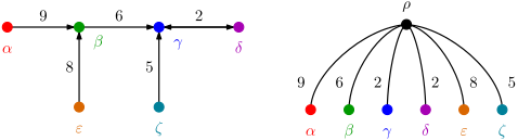
Figure 3.1: A component of \(F\) (left) becomes a node \(\rho\) with six children in \(H\) (right). Arrows show minimum-edge choices; the two selections of \(\gamma \delta\) give both \(\gamma\) and \(\delta\) a parent edge of weight \(2\).

All current vertices in a connected component of \(F\) become siblings under one new parent, even if its selected edges form a long chain. Thus a round adds one hierarchy level. The degrees in the hierarchy need not be binary: its vertices may have arbitrarily many children. We use this hierarchy directly for all subsequent query processing.

For a non-root hierarchy vertex \(v\), write \(\omega (v)\) for the weight of its parent edge. A hierarchy vertex represents a connected set of original vertices, namely its descendant leaves. An original edge selected in a round is contracted in that round, so it cannot label edges at two hierarchy levels. Its weight can occur twice only on sibling edges, when both endpoints select it. Consequently, the weights on any root-to-leaf path in \(H\) are distinct.

Lemma 3.2. The construction takes \(O(n)\) time and space. It produces a balanced hierarchy \(H\) with \(n\) leaves, fewer than \(2n\) vertices, and \(h\leq \lfloor \log n\rfloor\). If \(N_i\) is the number of vertices of height \(i\), then \(N_i\leq n/2^i\).

Proof. At any nonfinal round, the current graph is a tree with at least two vertices. Every vertex chooses an incident edge, so every component of \(F\) has at least two vertices. The next tree therefore has at most half as many vertices. A round scans only the current tree: find minima, traverse \(F\), and rebuild the remaining edge list in linear time in its current size. The total cost is a geometric series. Scanning the original graph or all original vertices in every round would not have this bound.

Each original leaf gets exactly one new ancestor per round. Hence all leaves have depth \(h\), and each internal vertex has at least two children. The total number of vertices is less than \(n+n/2+n/4+\cdots =2n\), and there are at most \(\lfloor \log n\rfloor\) rounds. A height-\(i\) vertex contains at least \(2^i\) leaves. Distinct vertices at that height have disjoint leaf sets, proving the bound on \(N_i\). □

Lemma 3.3. For every pair of distinct original vertices \(u,v\) (i.e., leaves of \(H\)), the maximum weight on \(P_H(u,v)\) is \(w_{T}^{}(u,v)\).

Proof. For one component of the selected forest \(F\) in one round, let \(r\) be its new hierarchy vertex and write \(\omega (C)=w(e_C)\) for each cluster \(C\). For distinct clusters \(C,D\), let \(e\) be the maximum-weight edge on their path. Since \(e\in F\), one of its endpoints selected it. An internal vertex of the path cannot select \(e\), because its other incident path edge is lighter. Thus \(C\) or \(D\) selected \(e\). Each endpoint’s selected minimum is no larger than its incident path edge, so

\[w(e)=\max \{\omega (C),\omega (D)\}.\]

This is exactly the maximum on the path \(C,r,D\) in the replacement star, proving that flattening preserves path maxima between clusters. See Figure 3.2.

Moving a surviving edge \(e\) from \(C\) to \(r\) leaves paths internal to \(C\) unaffected. Every affected path uses \(e\); since \(w(e)>\omega (C)\), adding or removing the lighter edge \(Cr\) leaves its maximum unchanged. Applying these rewritings round by round transforms \(T\) into \(H\) while preserving all path maxima between original vertices. □

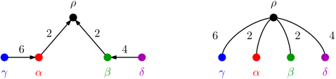
Figure 3.2: Flattening a selected component. On the left, the mutually selected edge of weight \(2\) has been split at \(\rho\). On the right, each cluster attaches to \(\rho\) with its selected weight, preserving all path maxima.

4 Splitting queries at lowest common ancestors

Lowest common ancestor (LCA) data structures admit reasonably simple constructions, such as that of Bender and Farach-Colton [BF00], with linear preprocessing time and space and constant query time. We use such a structure to preprocess the hierarchy \(H\). This is the only black box needed below. We work directly on \(H\) throughout the rest of the algorithm. For an integer \(0\leq q\leq d_v\), let \(v[q]\) denote the ancestor of \(v\) at depth \(q\); in particular, \(v[d_v]=v\). Since \(h\leq \lfloor \log n\rfloor\), a set of depths can be represented by a mask of \(h+1=O(\log n)\) bits.

Definition 4.1. For a query \((u_i,v_i)\), let \(\Delta _i\) be the depth of its LCA in \(H\). Split the path at this ancestor. Each of the two ancestor–leaf queries asks for the maximum edge weight from one endpoint up to the ancestor. Store one at each endpoint, with query depth \(\Delta _i\) and a reference to the original query.

Only the LCA’s depth is needed after this step. There are \(2s\) ancestor–leaf query records, and distinct query endpoints give \(0\leq \Delta _i<h\). Computing all query depths and storing the records takes \(O(s)\) time and space after preprocessing.

Observation 4.2. The two ancestor–leaf queries for \((u,v)\) partition the edges of \(P_H(u,v)\). Their maximum values therefore combine to \(w_{T}^{}(u,v)\).

5 Answering the queries at the leaves

Each ancestor–leaf query is stored and answered at its endpoint leaf \(v\). A record with query depth \(\Delta _i\) asks for the heaviest edge on the path from \(v[\Delta _i]\) to \(v\). We obtain these answers by a depth-first traversal of \(H\). At internal nodes, we maintain candidates for partial answers to queries at descendant leaves; reaching a leaf completes its answers.

5.1 Partial answers for descendant queries

Definition 5.1. For a non-root vertex \(v\) of \(H\), let \(\Pi _v\) be the set of ancestor–leaf query paths that use the parent edge of \(v\). Write \(u(P)\) for the upper endpoint of a path \(P\in \Pi _v\). The demand set at \(v\) is

\[D_v=\left\{ d_{u(P)} \;\middle\vert\; P\in \Pi _v \right\} \subseteq \{0,\ldots ,d_v-1\}.\]

Set \(\Pi _r=D_r=\varnothing\) at the root \(r\). For any vertex \(v\) and integer \(0\leq q\leq d_v\), the partial answer \(\mathop{\mathrm{suffix}}(q,v)\) is the weight of the heaviest edge on the path from \(v[q]\) to \(v\). The empty path at \(q=d_v\) has value \(-\infty\).

At a leaf \(v\), \(\mathop{\mathrm{suffix}}(\Delta _i,v)\) answers the stored ancestor–leaf query. At an internal node, \(\mathop{\mathrm{suffix}}(q,v)\) is the maximum over the part of that path reached so far. Candidate sets represent these values implicitly.

Each \(q\in D_v\) identifies the upper endpoint \(v[q]\). Store \(D_v\) as a bit mask, with one bit per distinct depth; the sets \(\Pi _v\) need not be stored. Compute the masks upward: collect query depths at leaves, and at each internal vertex \(v\) take the union of its children’s masks and discard all depths at least \(d_v\), by intersecting with \(\operatorname{Low}(d_v)\). A path with upper endpoint \(v\) contributes a demand below \(v\), but does not use the parent edge of \(v\). At each leaf, store all the queries associated with it.

While visiting \(v\), let \(\beta [t]=\omega (v[t])\) for \(1\leq t\leq d_v\): this is the weight of the parent edge of \(v[t]\). Adopt the lookup convention \(\beta [\bot ]=-\infty\) for an absent successor.

Definition 5.2. For a vertex \(v\) of \(H\), the candidate set \(S_v\) contains depths of non-root nodes on the root-to-\(v\) path. Each \(t\in S_v\) represents the parent edge of \(v[t]\). These edge weights strictly decrease as \(t\) increases, and

\[\beta [\mathop{\mathrm{succ}}(S_v,q)]=\mathop{\mathrm{suffix}}(q,v) \qquad \text {for every }q\in D_v.\]

Thus the first candidate deeper than \(q\) supplies the partial answer \(\mathop{\mathrm{suffix}}(q,v)\). At a leaf this is the requested answer. Extra candidates that represent no current demand are allowed.

Before the downward traversal, construct the table of Lemma 2.1 for the hierarchy height \(h\). Every demand depth is in \(\{0,\ldots ,h-1\}\), even though a candidate mask can also contain depth \(h\). The table indexes demand masks only. Since \(h\leq \lfloor \log n\rfloor\), its construction takes \(O(2^h)=O(n)\) time and space. No splitting into word fragments is needed.

5.2 Updating the candidates

Suppose a non-root node \(v\) has parent \(u\), depth \(d_v\), and parent edge \(uv\) of weight \(w=\omega (v)\). Extending the current path by this edge changes the partial answers, for \(q\in D_v\), according to

\[\mathop{\mathrm{suffix}}(q,v)=\max \{\mathop{\mathrm{suffix}}(q,u),w\}, \qquad q\in D_v.\]

To implement it, keep the shortest prefix of \(S_u\) containing the candidates for all demands whose old partial answers exceed \(w\), then append depth \(d_v\).

Let \(S=S_u\). The predicate \(P_v(q)=[\beta [\mathop{\mathrm{succ}}(S,q)]>w]\) is true on a prefix of \(D_v\), since the old partial answers are nonincreasing as \(q\) increases. Compute

\[q^*=\operatorname{LastTrue}(D_v,P_v).\]

Then set

\[k= \begin {cases} \mathop{\mathrm{succ}}(S,q^*), & q^*\ne -1,\ 0, & q^*=-1, \end {cases} \qquad S_v=(S\cap [k])\cup \{d_v\}. \tag{5.1}\]

Position zero is never a candidate, so \(k=0\) retains nothing. The intersection and union take constant time on masks, so the update takes constant time after finding \(q^*\).

Lemma 5.3. Starting with the empty set at the root, these updates preserve Definition 5.2.

Proof. Proceed by induction from the empty candidate set at the root. For a non-root node \(v\) with parent \(u\), the parent’s candidates represent the old answers for all \(q\in D_v\): inherited demands satisfy the invariant, and any new demand has \(q=d_u\), with both an empty partial path and no successor. By Lemma 2.2, \(\operatorname{LastTrue}\) is exact, so truncating at \(k\) retains the representative of every demand whose old answer exceeds \(w\), and every retained candidate has weight greater than \(w\). Consequently, every remaining demand has no retained successor and is represented by the appended candidate \(d_v\). Thus the update takes the maximum of each old answer and \(w\), while preserving strictly decreasing candidate weights. □

5.3 Completing the answers and implementing the traversal

Initialize \(M_i=-\infty\) for each query \(i\). Traverse \(H\) in depth-first order, starting with the empty candidate set at the root. At each non-root node \(v\), set \(\beta [d_v]=\omega (v)\) and perform Eq. (5.1). At an internal node, pass the resulting candidate set by value to each child. At a leaf \(v\), the partial answers are now complete: process each stored ancestor–leaf query by updating its original query’s answer:

\[M_i\gets \max \{M_i,\beta [\mathop{\mathrm{succ}}(S_v,\Delta _i)]\}.\]

Only leaves update the output values \(M_i\). After the traversal, return \(M_1,\ldots ,M_s\). The candidate invariant and Observation 4.2 give \(M_i=w_{T}^{}(u_i,v_i)\), proving the correctness assertion of Theorem 6.1. Passing the set by value preserves the parent’s state for its other children. The array \(\beta\) can be shared: a descendant writes only at a greater depth, and lookups use only depths on the current path.

6 Running time and space

Theorem 6.1. Under the model of Section 1, a tree with \(n\) vertices, distinct edge weights, and a batch of \(s\) path queries can be processed in deterministic \(O(n+s)\) time and \(O(n+s)\) space, including construction of the median table. The algorithm returns the path-maximum weight for every query. Consequently, MST verification, including all edge classifications, takes deterministic \(O(n+m)\) time and \(O(n+m)\) space.

Proof. Correctness was established in Section 5. We now prove the resource bounds. Put \(k_v=|D_v|\) and \(Q=2s\). At any height \(i\), charge each distinct demand to a descendant query record with that depth. The subtrees at one height are disjoint, so \(\sum _{v:h_v=i}k_v\leq Q\). There are \(N_i\leq n/2^i\) vertices at that height by Lemma 3.2.

Each search costs \(O(1+\log (k_v+1))\) by Lemma 2.2. Since \(\log (k+1)=O(\sqrt {k})\) for integers \(k\geq 0\), Cauchy–Schwarz bounds the nonconstant search work at height \(i\) by

\[\begin{align*} \sum _{v:h_v=i}\log (k_v+1) &=O\left (\sum _{v:h_v=i}\sqrt {k_v}\right )\\ &=O\left (\sqrt {N_i Q}\right ) =O\left (\sqrt {nQ}\,2^{-i/2}\right ). \end{align*}\]

Summing this geometric series and the constant overhead at the fewer than \(2n\) vertices gives \(O(n+\sqrt {nQ})=O(n+Q)\) time. Each predicate evaluation is constant-time: one successor lookup and at most one weight comparison. This accounts for the searches even when candidate sets contain unused elements.

The hierarchy and its LCA structure cost \(O(n)\) time and space. Computing query depths and storing both records costs \(O(s)\). Bottom-up unions, removal of depths at least the current depth, and candidate updates take constant time per hierarchy edge or vertex. Constructing the median table takes \(O(2^h)=O(n)\) time and space. Finally, decoding and accumulating the \(2s\) ancestor–leaf answers costs \(O(s)\). This accounts for all work and gives deterministic \(O(n+s)\) total time.

The hierarchy, LCA structure, demands, and candidate state occupy \(O(n)\) words. The weight array \(\beta\) and traversal stack need \(O(h+1)=O(\log n)\) words; the query records and answers need \(O(s)\). No search materializes a list of its set bits. Including the median table, the space bound is \(O(n+s)\).

MST verification. First check in \(O(n+m)\) time that the proposed edges form a spanning tree. For a valid proposal, query every non-tree, non-loop edge and compare its weight with its returned path maximum. This gives all lighter, equal, or heavier classifications; each tree edge has its own weight as its path maximum, and loops are marked separately. By the cycle criterion, the proposed tree is minimum exactly when no edge is lighter than its path maximum. This takes deterministic \(O(n+m)\) time and \(O(n+m)\) space. □

References

[BF00] Michael A. Bender and Martín Farach-Colton. “The LCA Problem Revisited”. In: LATIN 2000: Theoretical Informatics. Vol. 1776. Lecture Notes in Computer Science. Springer, 2000, pp. 88–94. doi: 10.1007/10719839_9.

[Hag10] Torben Hagerup. “An Even Simpler Linear-Time Algorithm for Verifying Minimum Spanning Trees”. In: Graph-Theoretic Concepts in Computer Science. Ed. by Christophe Paul and Michel Habib. Vol. 5911. Lecture Notes in Computer Science. WG 2009. Springer, 2010, pp. 178–189. doi: 10.1007/978-3-642-11409-0_16.

[Kin97] Valerie King. “A Simpler Minimum Spanning Tree Verification Algorithm”. In: Algorithmica 18 (1997), pp. 263–270. doi: 10.1007/BF02526037.

[Zwi09] Uri Zwick. Verification of Minimum Spanning Trees. Lecture notes for “Advanced Graph Algorithms”, Tel Aviv University. 2009. url: https://www.cs.tau.ac.il/~zwick/grad-algo-0910/mst-verify.pdf.